Why are nanoelectronic devices interesting?

1. A supercomputer in your hands#

Klimeck opens with a comparison. The fastest supercomputer of 1985, the Cray-2, and the iPad 2 of 2011 both deliver about 4 GFLOPS, i.e. \(4\times10^9\) floating-point operations (multiplications and additions of floating-point numbers) per second. The Cray needed a custom room that could carry it, chilled-water cooling, controlled access and specially trained users; the tablet is handed to children who are just learning to read, and has been taken along to the International Space Station. To give the Cray's size a feeling he compares it with his family minivan: about the same mass, 2,500 kg fully loaded, and about the same power, 195 kW.

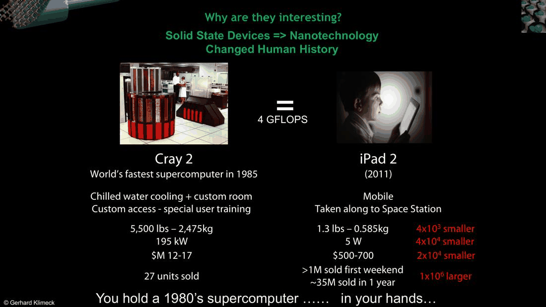
The cell below computes the ratios on the slide from its data (the price ranges are taken at their midpoints).

The tablet is about four thousand times lighter, forty thousand times less power hungry and twenty thousand times cheaper, and it sold a million times more units: over a million in its first weekend and about 35 million in its first year, against 27 Cray-2 machines. Since both compute at the same rate, the energy per floating-point operation dropped by the power ratio, \(3.9\times10^4\).

2. Modern society runs on nanotechnology#

The same semiconductor technology runs communications, every business operation, manufacturing and agriculture. Klimeck's second example is not a processor at all: radio-frequency identification (RFID) tags, in credit cards, toll tags and ski passes. They secure financial transactions, and 76 billion of them were sold in 2018 — a short-term commodity that is thrown away. Such numbers are only possible because each device costs almost nothing.

3. Moore's law#

In 1965 Gordon Moore sketched the relative manufacturing cost per component against the number of components per integrated circuit. For each year the curve has a minimum: putting more components on a chip lowers the cost per component, until yield problems produce diminishing returns. Over the years the minimum moves to more components and lower cost. Read today, the law is usually stated as the number of transistors per chip doubling about every two years.

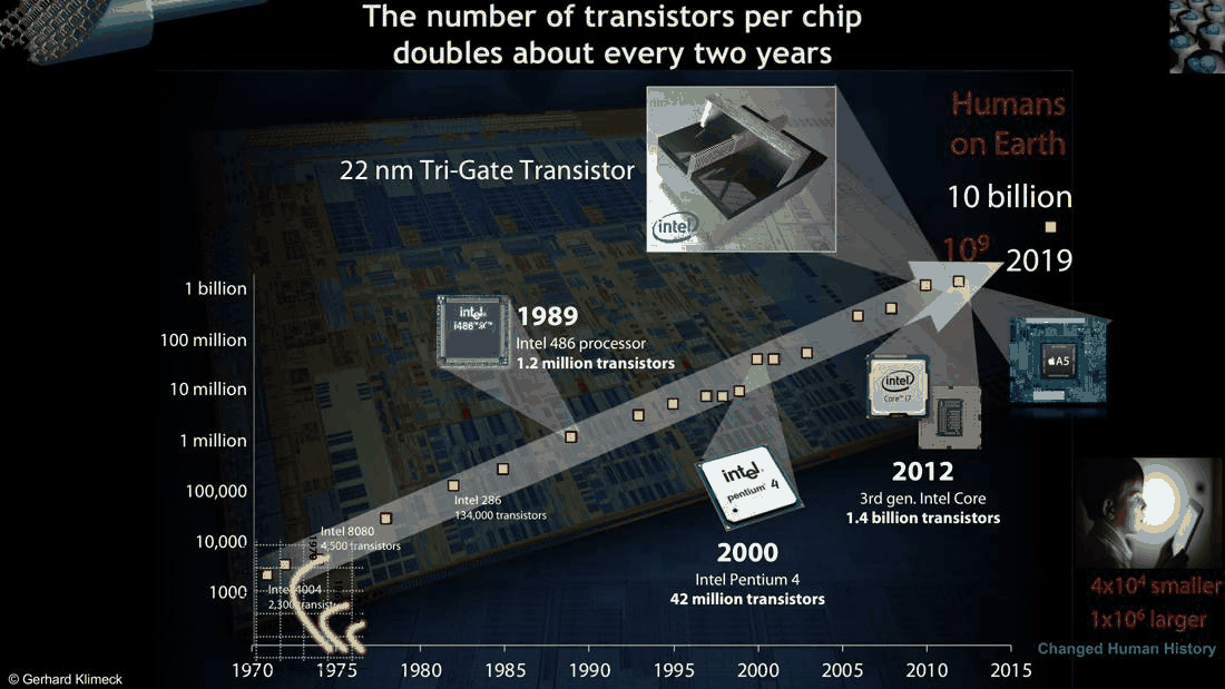
If \(N(t) = N_0\,2^{(t - t_0)/\tau}\), then \(\log_2 N\) is a straight line in \(t\) with slope \(1/\tau\). The cell fits the six processors labelled on the slide.

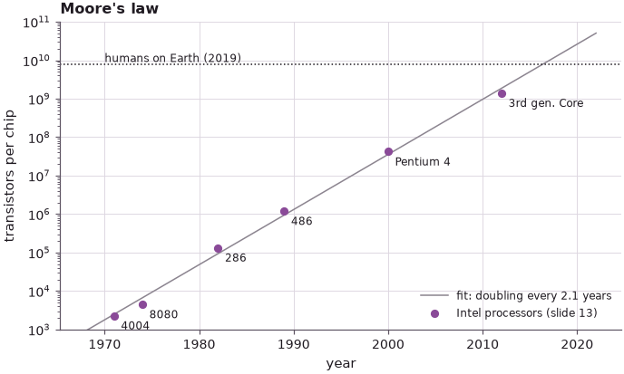
The six processors give a doubling time of a little over two years, and over 41 years a growth by a factor of about \(6\times10^5\), i.e. almost twenty doublings. Klimeck stresses what the end point means: more transistors on one die than people on the planet, all of them working together without a fault. That is as much a statement about the quality of the design as about the size of the number.

4. Devices are atomically small#

Making the transistors smaller is what puts more of them on a chip and lowers the cost of each. The "technology node" (22 nm, 14 nm, ...) roughly names the gate length. In 2012 Intel's 22 nm node introduced the first mass-produced three-dimensional transistor, the tri-gate or FinFET: a thin silicon fin is the channel, and the gate wraps around it on three sides. Klimeck's picture is a garden hose: electrons enter from the source, flow through the channel, and the gate is a valve that squeezes the hose shut or opens it.

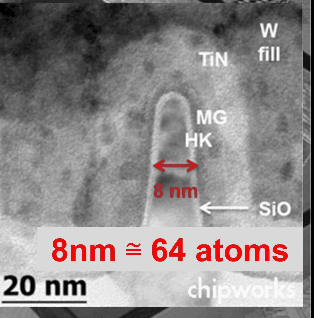
Eight nanometres is a number of atoms one can count. It is not Avogadro's number of particles but a few dozen, so the channel is no longer a continuum material: "Atomistically small. That means it's not continuum material. You really have to understand quantum mechanics." For comparison, a red blood cell is about 7,000 nm across, 875 times the fin width.

open-nemo builds the silicon crystal from the lattice constant of its tight-binding parameter set. The cell counts the atomic planes that fit across 8 nm for two directions a fin's width can take: along [001], where the planes are \(a/4\) apart, and along [110], where they are \(a\sqrt{2}/4\) apart.

Across 8 nm there are 59 (001) planes or 42 (110) planes: a few dozen atoms, the same order as the slide's 64, which counts eight atoms per nanometre.

When does an electron notice the confinement?#

A first quantitative answer: confine silicon to a film of thickness \(t\) and compute the lowest conduction-band state. In the effective-mass picture the film is a particle in a box with infinite walls, and the lowest subband of the two valleys whose heavy (longitudinal) mass \(m_l = 0.916\,m_0\) points across the film lies

above the bulk conduction-band minimum. The atomistic answer comes from the sp3d5s* tight-binding model of Boykin et al. (2004): open-nemo builds (001) films of 2 to 15 conventional cells, periodic in the plane and terminated by hydrogen-like passivation, and the cell takes the lowest conduction state at the in-plane Γ point (where the two valleys along [001] fold). The thermal energy \(k_BT = 25.9\) meV at 300 K is the scale to compare with: a confinement energy well below it barely changes the electron population; one well above it does.

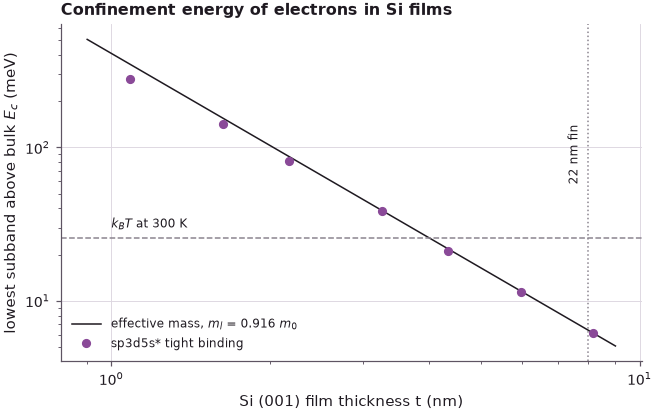
At the 8 nm of the 22 nm node the confinement raises the lowest state by about 6 meV, a quarter of \(k_BT\): noticeable, but the particle-in-a-box formula still describes it to within a few percent. Below about 4 nm the shift exceeds \(k_BT\), and at 1.1 nm (16 atoms per in-plane cell) it is roughly ten times \(k_BT\); there tight binding and the effective-mass formula part ways (by about 20 % at 1.1 nm), because the electron samples the band far from its minimum, where it is no longer parabolic. The fins of the later nodes (about 6 nm and fewer atoms, see Lecture 2) and nanosheets a few nanometres thick sit in the range where this matters. Lecture 1.3 returns to why the parabolic band fails, and Section 9 of the course to what the atoms do to the states.

5. Transistors became 100 million times cheaper#

The last argument is economic. The website Our World in Data collects inflation-adjusted price histories of many products, some going back to 1930. Milk and sugar cost about the same throughout; polyester fibre, wind turbines and cars changed comparatively little. The transistor is the outlier: its price fell by a factor of about \(10^8\). Only a few other products came close — DRAM, the hard disk drive and DNA sequencing; laser diodes started on a similar slope but levelled off, and photovoltaics fell more slowly.

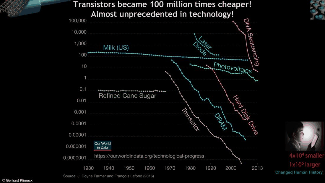
On the chart the transistor curve runs from about 1968 to the mid-2000s, roughly 40 years. Spread over 35–45 years, a factor \(10^8\) is a constant yearly reduction of:

Over 40 years the price per transistor halves every 1.5 years (1.3–1.7 years for 35–45 years), faster than the transistor count doubles. This is the sense in which the technology changed human history: transistors are affordable to essentially everyone, so they can be in everything — communication, computing and every part of society.

6. Learning objectives#

A typical solid-state devices course (Klimeck teaches one at Purdue) aims to explain the working principles and the physical processes of these devices, to relate device performance to materials and design criteria, to speak the language of device engineers and to be ready to engage in device research. This course adds what such courses usually leave out:

• understand band structure,
• understand the atomistic transport issues in modern devices,
• operate advanced simulation tools for device exploration.

The next lecture (1.2) starts from the basic operation of a transistor and the many questions its textbook pictures raise.

Summary#

• A 2011 tablet matches a 1985 supercomputer's 4 GFLOPS while being about \(4\times10^3\) times lighter, \(4\times10^4\) times less power hungry and \(2\times10^4\) times cheaper; it sold \(10^6\) times more units.
• The six Intel processors on slide 13 give a doubling time of the transistor count of a little over two years; by 2019 a chip held about \(10^{10}\) transistors.
• The 8 nm fin of the 22 nm tri-gate transistor is a few dozen atomic planes wide (59 along [001], 42 along [110] in open-nemo's Si crystal).
• In an 8 nm Si film the confinement raises the lowest electron state by about 6 meV, a quarter of \(k_BT\); below about 4 nm it exceeds \(k_BT\) and the parabolic-band estimate starts to fail.
• A price drop of \(10^8\) over about 40 years is a halving every 1.5 years.

Exercises#

1. Repeat the doubling-time fit with only the processors before 1990, and with only those after. Has the pace changed?
2. Extend the film table to 20 and 30 conventional cells (10.9 and 16.3 nm) and check that the tight-binding shift approaches the effective-mass formula. Why does the code above build only films that are a whole number of conventional cells thick?
3. Repeat the film calculation for the Δ valleys lying in the plane of the film, whose mass across the film is \(m_t = 0.19\,m_0\) (search the lowest conduction state at in-plane \(k \approx 0.15 \times 2\pi/a\) along y). Which valleys are lowest in a thin film, and why?
4. How many silicon atoms are in a fin 8 nm wide, 40 nm tall and 22 nm long? (Si has 8 atoms per conventional cell of volume \(a^3\).)

Further reading#

• Crystal structures, reciprocal lattices and Brillouin zones
• Ultra-thin bodies: subbands versus thickness, orientation and material
• FinFETs and nanosheets
• G. E. Moore, "Cramming more components onto integrated circuits", Electronics 38, 114 (1965).
• J. D. Farmer and F. Lafond, "How predictable is technological progress?", Research Policy 45, 647 (2016); data at ourworldindata.org/technological-progress.
• T. B. Boykin, G. Klimeck and F. Oyafuso, Phys. Rev. B 69, 115201 (2004) (the sp3d5s* Si parameters).