Lecture 10.2

Introduction to transport — a simple rate-equation model of sequential tunneling

In the lecture

the simplest transport model, before any wave mechanics: a single level between two reservoirs, filled and emptied at hopping rates $\Gamma_L/\hbar$ and $\Gamma_R/\hbar$
the rate equation for its occupation $n$: in-flow minus out-flow through each barrier
the steady state: $n = (\Gamma_Lf_L + \Gamma_Rf_R)/(\Gamma_L + \Gamma_R)$ and the current $I = (e/\hbar)\,\Gamma_L\Gamma_R/(\Gamma_L + \Gamma_R)\,(f_L - f_R)$
intuitive limits: the thick barrier limits the current; asymmetric coupling decides whether the level is full or empty, and so influences the voltage drop in the device
the link to the Landauer formula of the next lecture

In this notebook

you take the hopping rates $\Gamma_L$ and $\Gamma_R$ of real GaAs/AlGaAs double barriers from open-nemo's resonance solver, integrate the rate equation in time, check the steady-state occupation and current in the lecture's limits, compute the current–voltage curve of a level that moves with the bias, and show that the Landauer formula with a Lorentzian transmission gives the same current.

Run the notebookEvery number and figure on this page comes from it. Change it, rerun it, take it further.

Download .ipynb View on GitHub

Run it on your own machine

The notebook needs open-nemo (Python ≥ 3.10 and a C++20 compiler; BLAS/LAPACK).

git clone https://github.com/denphi/open-nemo.git && cd open-nemo
python3 -m venv .venv && source .venv/bin/activate
pip install -e ".[notebooks]"
jupyter lab From_Atoms_to_Devices/05_introduction_to_transport/10_2_sequential_tunneling_rate_equations.ipynb

Code10 lines · cell 1

import numpy as np
import matplotlib.pyplot as plt
from scipy.integrate import solve_ivp
import opennemo as nemo
from opennemo.visualization import style
from opennemo.structures.statistics import fermi

style.use(notebook=True)
EM = nemo.structures.materials.EffectiveMassMaterial
Q, HBAR = nemo.core.units.Q, nemo.core.units.HBAR      # C, eV s

1. The simplest transport model: a rate equation for one level#

Klimeck starts from the conceptual picture of Lecture 10.1 (two reservoirs, an object with channels) and reduces the object to a single quantum state at the resonance energy $E_r$. The reservoirs are filled according to Fermi functions $f_{L,R}(E) = 1/(1 + e^{(E - \mu_{L,R})/k_BT})$ with chemical potentials $\mu_L$ and $\mu_R = \mu_L - eV$, separated by the applied voltage $V$. An electron hops between the level and the left reservoir at the rate $\Gamma_L/\hbar$ (per second) and between the level and the right reservoir at $\Gamma_R/\hbar$; $\Gamma_{L,R}$ are energies. The level can move with the bias, $E_r(\alpha V)$, where $\alpha$ describes how much of the voltage drops before the level ("the state may not be exactly going down at a rate of half").

Slide 4: a rate equation for one level — Slide 4: the single level between two reservoirs, the hopping rates and the symbols of the model.

The occupation $n$ of the level changes by hopping in minus hopping out, through each barrier:

\frac{dn}{dt} = \frac{\Gamma_L}{\hbar}\bigl[f_L(E_r) - n\bigr] + \frac{\Gamma_R}{\hbar}\bigl[f_R(E_r) - n\bigr].

The term $\Gamma_Lf_L/\hbar$ is the in-flow from the left (proportional to how many electrons the left contact offers at $E_r$), $\Gamma_Ln/\hbar$ the out-flow back to the left; the right side is the same. No wave mechanics enters: the rates are inputs. Wave mechanics (Lecture 10.3) tells where they come from: they are the widths of the quasi-bound state when only one barrier lets it leak. Here $\Gamma_L$ is computed with nemo.resonances for a structure whose right barrier is made 14 nm thick (so that the state leaks only to the left), and $\Gamma_R$ the other way round. The structures are GaAs wells of 5 nm with Al$x$Ga${1-x}$As barriers 0.3 eV high (masses $0.067\,m_0$ and $0.092\,m_0$); the barrier thicknesses $b_L$ and $b_R$ vary.

Code24 lines · cell 3

gaas = EM("GaAs", 0.067, 12.9)
algaas = EM("AlGaAs", 0.092, 12.2, conduction_band_edge=0.3)


def double_barrier(b_left, b_right, well=5.0, lead=10.0, dx=0.05):
    mats = (gaas, algaas, gaas, algaas, gaas)
    widths = (lead, b_left, well, b_right, lead)
    return nemo.Heterostructure1D([nemo.Layer(m, d) for m, d in zip(mats, widths)], spacing=dx)


def rates(b_left, b_right):
    # lowest resonance energy and its width (eV): full structure, left barrier only, right barrier only
    res = nemo.resonances(double_barrier(b_left, b_right))
    gl = nemo.resonances(double_barrier(b_left, 14.0))["width"][0]
    gr = nemo.resonances(double_barrier(14.0, b_right))["width"][0]
    return res["energy"][0], res["width"][0], gl, gr


rate_table = {}
print(" b_L  b_R (nm)   E_r (meV)   Γ (meV)   Γ_L (meV)   Γ_R (meV)   Γ_L + Γ_R (meV)")
for bl, br in ((5, 5), (4, 6), (3, 5), (5, 3)):
    er, g, gl, gr = rate_table[bl, br] = rates(bl, br)
    print(f"  {bl}    {br}        {er * 1e3:6.2f}    {g * 1e3:7.4f}    {gl * 1e3:7.4f}"
          f"     {gr * 1e3:7.4f}        {(gl + gr) * 1e3:7.4f}")

 b_L  b_R (nm)   E_r (meV)   Γ (meV)   Γ_L (meV)   Γ_R (meV)   Γ_L + Γ_R (meV)
  5    5         81.79     0.1293     0.0647      0.0647         0.1293
  4    6         81.76     0.2911     0.2760      0.0151         0.2912
  3    5         81.60     1.2413     1.1774      0.0647         1.2421
  5    3         81.60     1.2413     0.0647      1.1774         1.2421

The width of the full structure equals the sum $\Gamma_L + \Gamma_R$ of the one-sided widths to better than 0.1 %: the escape rates through the two barriers add. A 1 nm thinner barrier increases its rate by a factor of about 4.3 (compare $\Gamma_R$ for 5 and 6 nm with $\Gamma_L$ for 4 nm and 5 nm), the exponential sensitivity of tunneling.

The rate equation is linear in $n$ and relaxes exponentially to its steady state with the time constant $\tau = \hbar/(\Gamma_L + \Gamma_R)$. Below it is integrated numerically for the asymmetric 3 nm | 5 nm structure at large bias ($f_L = 1$, $f_R = 0$), starting from an empty level, together with the currents through the left and the right barrier,

I_L = \frac{e}{\hbar}\Gamma_L\,(f_L - n),\qquad I_R = \frac{e}{\hbar}\Gamma_R\,(n - f_R).

Code32 lines · cell 5

er, g, gl, gr = rate_table[3, 5]
fl, fr = 1.0, 0.0
tau = HBAR / (gl + gr)


def dndt(t, n):
    return gl / HBAR * (fl - n) + gr / HBAR * (fr - n)


t = np.linspace(0, 10 * tau, 500)
sol = solve_ivp(dndt, (0, t[-1]), [0.0], t_eval=t, rtol=1e-10, atol=1e-12)
n_t = sol.y[0]
n_ss = (gl * fl + gr * fr) / (gl + gr)
n_exact = n_ss * (1 - np.exp(-t / tau))
print(f"τ = ħ/(Γ_L + Γ_R) = {tau * 1e12:.3f} ps")
print(f"steady state n = {n_ss:.4f}; numerical n(10τ) = {n_t[-1]:.4f};"
      f" largest |n_numerical - n_exact| = {abs(n_t - n_exact).max():.1e}")
IL = Q / HBAR * gl * (fl - n_t) * 1e9
IR = Q / HBAR * gr * (n_t - fr) * 1e9
print(f"at t = 0:  I_L = {IL[0]:.2f} nA, I_R = {IR[0]:.2f} nA;  at t = 10τ: I_L = {IL[-1]:.3f} nA,"
      f" I_R = {IR[-1]:.3f} nA (per spin)")

fig, axes = plt.subplots(1, 2, figsize=(10, 3.6))
axes[0].plot(t * 1e12, n_t, color=style.OPEN_NEMO, label="solve_ivp")
axes[0].plot(t * 1e12, n_exact, ":", color=style.REFERENCE, label="n∞(1 − e^(−t/τ))")
axes[0].set(xlabel="time (ps)", ylabel="occupation n", title="filling the level, 3 nm | 5 nm")
axes[0].legend(frameon=False, fontsize=8)
axes[1].semilogy(t * 1e12, IL, color=style.OPEN_NEMO, label="through the left barrier")
axes[1].semilogy(t * 1e12, IR, color=style.CONTEXT, label="through the right barrier")
axes[1].set(xlabel="time (ps)", ylabel="current per spin (nA)", title="in-flow and out-flow")
axes[1].legend(frameon=False, fontsize=8)
fig.tight_layout()

τ = ħ/(Γ_L + Γ_R) = 0.530 ps
steady state n = 0.9479; numerical n(10τ) = 0.9479; largest |n_numerical - n_exact| = 1.9e-11
at t = 0:  I_L = 286.60 nA, I_R = 0.00 nA;  at t = 10τ: I_L = 14.933 nA, I_R = 14.920 nA (per spin)

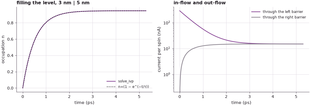
Figure computed by the notebook with open-nemo

The level fills within a few $\tau = 0.530$ ps up to $n = 0.948$. At first the left barrier lets 287 nA flow in while nothing flows out; the difference charges the level. In the steady state the two currents are equal, 14.92 nA per spin: whatever comes in from the left leaves to the right.

2. The steady state: occupation and current#

With $dn/dt = 0$ the rate equation gives the occupation, and the current through the right barrier follows:

n = \frac{\Gamma_Lf_L + \Gamma_Rf_R}{\Gamma_L + \Gamma_R},\qquad I = \frac{e}{\hbar}\,\frac{\Gamma_L\Gamma_R}{\Gamma_L + \Gamma_R}\,(f_L - f_R)\quad(\times 2\text{ for spin}).

The occupation is the in-flow divided by the total out-flow rate: a balance of in-flow over out-flow. The current has the form that will recur throughout the course: a product of the two rates over their sum (like two conductances in series) times the difference of the occupations of the contacts.

3. Intuitive limits#

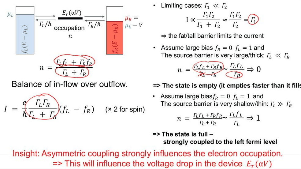
Slide 5: limits of the rate equation — Slide 5: the limiting cases. The thick (or tall) barrier limits the current; at large bias a thin source barrier fills the level and a thick one leaves it empty.

If one rate is much smaller, $\Gamma_1 \ll \Gamma_2$, then $I \propto \Gamma_1\Gamma_2/(\Gamma_1 + \Gamma_2) \approx \Gamma_1$: the fat or tall barrier limits the current.
At large bias ($f_L = 1$, $f_R = 0$) with a thick source barrier, $\Gamma_L \ll \Gamma_R$: $n \approx \Gamma_L/\Gamma_R \to 0$. The level empties faster than it fills.
At large bias with a thin source barrier, $\Gamma_L \gg \Gamma_R$: $n \to 1$. The level is full, strongly coupled to the left Fermi level.

The table applies these formulas to the four computed structures at large bias, including spin.

Code16 lines · cell 7

print(" b_L  b_R (nm)   Γ_L/Γ_R    n (large bias)   I = 2(e/ħ) Γ_LΓ_R/(Γ_L+Γ_R) (nA)   2(e/ħ) min(Γ) (nA)")
for (bl, br), (er, g, gl, gr) in rate_table.items():
    n = gl / (gl + gr)
    I = 2 * Q / HBAR * gl * gr / (gl + gr)
    print(f"  {bl}    {br}       {gl / gr:7.3f}       {n:.4f}               {I * 1e9:7.2f}"
          f"                      {2 * Q / HBAR * min(gl, gr) * 1e9:7.2f}")

ratio = np.logspace(-3, 3, 200)
g_sum = 1.0
gl_r, gr_r = g_sum * ratio / (1 + ratio), g_sum / (1 + ratio)
fig, ax = plt.subplots(figsize=(6.5, 3.6))
ax.semilogx(ratio, gl_r / g_sum, color=style.OPEN_NEMO, label="occupation n")
ax.semilogx(ratio, 4 * gl_r * gr_r / g_sum**2, color=style.CONTEXT,
            label="current / its maximum, 4Γ_LΓ_R/(Γ_L+Γ_R)²")
ax.set(xlabel="Γ_L / Γ_R", ylabel="normalized", title="large bias, fixed Γ_L + Γ_R")
ax.legend(frameon=False, fontsize=8);

 b_L  b_R (nm)   Γ_L/Γ_R    n (large bias)   I = 2(e/ħ) Γ_LΓ_R/(Γ_L+Γ_R) (nA)   2(e/ħ) min(Γ) (nA)
  5    5         1.000       0.5000                 15.74                        31.48
  4    6        18.222       0.9480                  6.99                         7.37
  3    5        18.208       0.9479                 29.84                        31.48
  5    3         0.055       0.0521                 29.84                        31.48

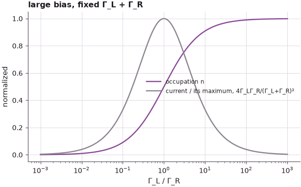
The symmetric 5 nm | 5 nm structure is half full ($n = 0.5000$). Thinning the source barrier to 3 nm makes $\Gamma_L/\Gamma_R = 18.2$ and fills the level to $n = 0.948$; the reverse structure, 5 nm | 3 nm, has the same current (the formula is symmetric in the two rates) but an almost empty level, $n = 0.052$. For both asymmetric pairs the current is 5 % below the value set by the smaller rate alone.

Klimeck's insight is the last point: asymmetric coupling strongly influences the electron occupation, and the occupation is charge. A full level in the well charges it and raises the potential there, so it changes the voltage drop through the device, which in turn moves $E_r(\alpha V)$. Current, charge and potential depend on each other; Lectures 10.5 and 10.6 close that loop.

4. Current through a level that moves with the bias#

The level moves down with the bias, $E_r(V) = E_r(0) - \alpha eV$. With $\mu_L = 50$ meV above the emitter conduction-band edge and $\mu_R = \mu_L - eV$, the Fermi functions $f_L(E_r)$ and $f_R(E_r)$ switch the current on when the level crosses $\mu_L$, at $V = (E_r(0) - \mu_L)/\alpha e$. The rates of the symmetric 5 nm | 5 nm structure are used, with $\alpha = 0.5$ (the level in the middle of a symmetric drop) and $\alpha = 0.3$.

Code18 lines · cell 9

er0, g, gl, gr = rate_table[5, 5]
mu_l = 0.05
V = np.linspace(0, 0.3, 601)
fig, axes = plt.subplots(1, 2, figsize=(10, 3.6))
for alpha, c in zip((0.5, 0.3), (style.OPEN_NEMO, style.CONTEXT)):
    er = er0 - alpha * V
    for temp, ls in ((4, "-"), (300, "--")):
        fl, fr = fermi(er, mu_l, temp), fermi(er, mu_l - V, temp)
        n = (gl * fl + gr * fr) / (gl + gr)
        I = 2 * Q / HBAR * gl * gr / (gl + gr) * (fl - fr) * 1e9
        axes[0].plot(V, I, ls, color=c, label=f"α = {alpha}, {temp} K")
        axes[1].plot(V, n, ls, color=c)
    print(f"α = {alpha}: onset at (E_r - μ_L)/α = {(er0 - mu_l) / alpha:.3f} V,"
          f" saturation current {2 * Q / HBAR * gl * gr / (gl + gr) * 1e9:.2f} nA")
axes[0].set(xlabel="bias V (V)", ylabel="current (nA)", title="rate equation, 5 nm | 5 nm")
axes[0].legend(frameon=False, fontsize=8)
axes[1].set(xlabel="bias V (V)", ylabel="occupation n", title="occupation of the level")
fig.tight_layout()

α = 0.5: onset at (E_r - μ_L)/α = 0.064 V, saturation current 15.74 nA
α = 0.3: onset at (E_r - μ_L)/α = 0.106 V, saturation current 15.74 nA

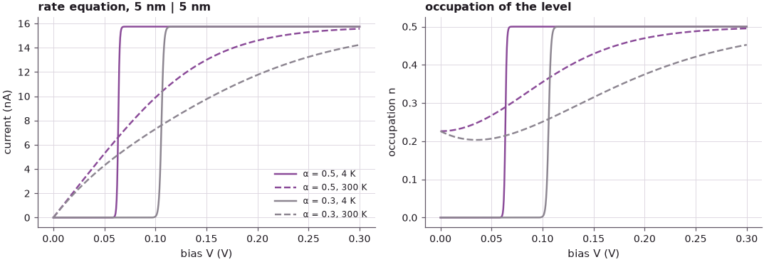
At 4 K the current switches on at 0.064 V for $\alpha = 0.5$ and at 0.106 V for $\alpha = 0.3$, as a step to 15.74 nA, and the occupation steps from 0 to $\Gamma_L/(\Gamma_L + \Gamma_R) = 0.5$. At 300 K the steps are smeared over a few $k_BT/\alpha$, and the level is partly occupied even at zero bias, because both contacts fill it in equilibrium.

What this simple model lacks is also instructive. Once switched on, the current stays constant, while the coherent calculation of Lecture 10.1 for the same structure shows a peak and a drop (negative differential resistance). The reason is that $\Gamma_L$ is not a constant: when the level falls below the conduction-band edge of the emitter, there are no states left to tunnel from and $\Gamma_L$ vanishes. Wave mechanics supplies $E_r$ and $\Gamma$ as functions of the bias, as Klimeck says at the end: "the rate equations gave us the shape of the answers and the wave mechanics will tell us how we can calculate gammas and eigenenergies".

5. Connecting the rate equation to Landauer transport#

The Landauer formula of Lecture 10.1, $I = (2e/h)\int T(E)\,[f_L(E) - f_R(E)]\,dE$, describes the same structure through a transmission. Near an isolated resonance the transmission is a Lorentzian (the Breit–Wigner form, derived in Lecture 10.3),

T(E) = \frac{\Gamma_L\Gamma_R}{(E - E_r)^2 + (\Gamma_L + \Gamma_R)^2/4},\qquad \int T(E)\,dE = \frac{2\pi\,\Gamma_L\Gamma_R}{\Gamma_L + \Gamma_R}.

If the resonance is much narrower than $k_BT$, the Fermi functions are constant across it, and the Landauer integral becomes $(2e/h)\cdot 2\pi\,\Gamma_L\Gamma_R/(\Gamma_L + \Gamma_R)\cdot(f_L - f_R)$, which is exactly the rate-equation current with spin, since $2\pi/h = 1/\hbar$. The check below uses nemo.landauer_current with the Lorentzian of the 3 nm | 5 nm structure at 300 K.

Code12 lines · cell 11

er0, g, gl, gr = rate_table[3, 5]
gam = gl + gr
E = np.unique(np.concatenate([np.linspace(-0.3, 0.6, 4001), er0 + gam * np.linspace(-200, 200, 8001)]))
print("  E_r - μ_L (meV)   I Landauer, Lorentzian T (nA)   I rate equation (nA)   ratio")
for d in (-60, -20, 0, 20, 60):
    mu_l = er0 - d * 1e-3
    mu_r = mu_l - 0.1
    T_bw = gl * gr / ((E - er0) ** 2 + gam**2 / 4)
    I_l = nemo.landauer_current(E, T_bw, mu_l, mu_r, 300)
    I_r = 2 * Q / HBAR * gl * gr / gam * (fermi(er0, mu_l, 300) - fermi(er0, mu_r, 300))
    print(f"        {d:4d}               {I_l * 1e9:9.4f}                  {I_r * 1e9:9.4f}"
          f"         {I_l / I_r:.4f}")

  E_r - μ_L (meV)   I Landauer, Lorentzian T (nA)   I rate equation (nA)   ratio
         -60                 21.7387                    21.9373         0.9909
         -20                 18.9752                    19.1280         0.9920
           0                 14.2392                    14.3102         0.9950
          20                  9.1443                     9.1360         1.0009
          60                  2.6651                     2.6070         1.0223

The two currents agree to within 2.3 % here, with $\Gamma_L + \Gamma_R = 1.24$ meV, 21 times smaller than $k_BT = 25.9$ meV. The small difference comes from the Lorentzian tails, which reach out to where the Fermi functions do change. Lecture 10.4 compares the sequential and coherent pictures in detail, including the case where they part company.

Summary#

A single level coupled to two reservoirs at rates $\Gamma_{L,R}/\hbar$ obeys $dn/dt = (\Gamma_L/\hbar)(f_L - n) + (\Gamma_R/\hbar)(f_R - n)$; it relaxes to its steady state in $\tau = \hbar/(\Gamma_L + \Gamma_R)$, about half a picosecond for the 3 nm | 5 nm structure.
Steady state: $n = (\Gamma_Lf_L + \Gamma_Rf_R)/(\Gamma_L + \Gamma_R)$ and $I = 2(e/\hbar)\,\Gamma_L\Gamma_R/(\Gamma_L + \Gamma_R)\,(f_L - f_R)$ with spin.
The thicker barrier limits the current; at large bias a thin source barrier fills the level and a thick one empties it. The occupation is charge and will change the voltage drop.
The rates are widths of quasi-bound states: open-nemo's resonance widths for one-sided structures add up to the width of the double barrier.
For a resonance narrower than $k_BT$, the Landauer formula with a Lorentzian transmission gives the rate-equation current.

Exercises#

Repeat the time integration of Section 1 for the 5 nm | 3 nm structure. How do the initial currents and the steady-state occupation change, and why is the steady-state current the same?
Make $\Gamma_L$ depend on the bias in Section 4: set it to zero once $E_r(V)$ falls below the emitter band edge (0 eV). Compare the resulting I–V with the coherent result of Lecture 10.1.
In Section 5, increase $\Gamma_L$ and $\Gamma_R$ by factors of 10 and 100 (keeping their ratio). At which width does the rate equation differ from the Landauer current by more than 10 %?