

ECE 606 Lecture 6.5
Analytical and numerical solution strategies
In the lecture
- the analytical route for closed systems: five steps from an ansatz to a determinant whose zeros are the energies
- the transfer-matrix method for open systems: simple and appealing, but limited to flat potentials and a moderate number of thin layers
- discretizing the Schrödinger equation on a grid: the three-point second derivative from a Taylor expansion, \(t_0 = \hbar^2/(2ma^2)\)
- the Hamiltonian as a tridiagonal matrix and the energies as its eigenvalues, the same structure as a tight-binding chain with one s orbital per site
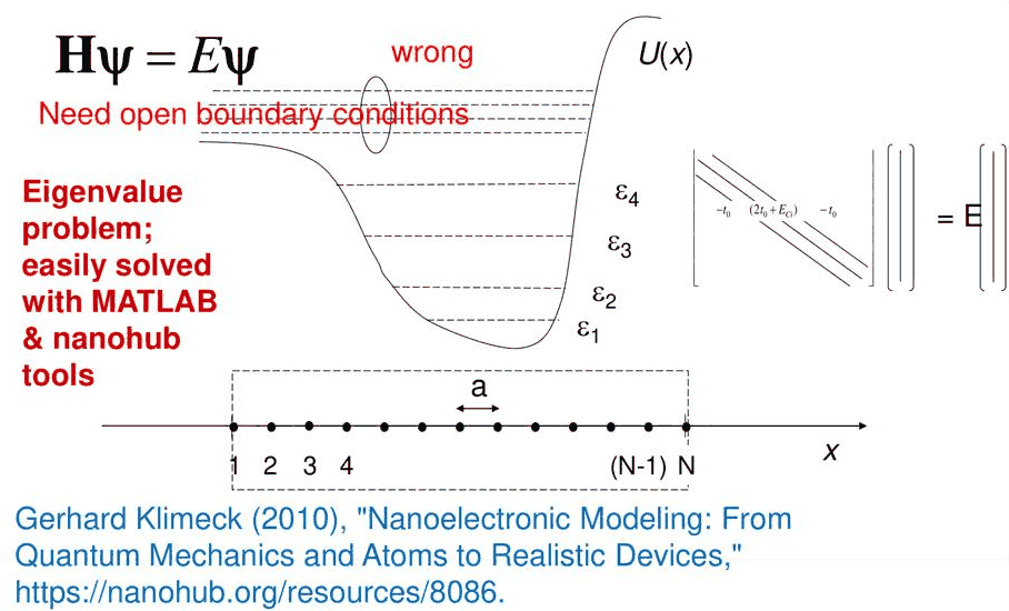
- closed boundary conditions give wrong answers for devices from which electrons leak out: open boundary conditions are needed
In this notebook
solves a finite well with the five-step determinant, shows where the transfer matrix needs slicing and where it loses precision, builds the finite-difference Hamiltonian by hand and checks it against open-nemo's, measures its discretization error, compares a closed box with the open system, and explores how a position-dependent mass must be discretized.
Run it on your own machine
The notebook needs open-nemo (Python ≥ 3.10 and a C++20 compiler; BLAS/LAPACK).
git clone https://github.com/denphi/open-nemo.git && cd open-nemo
python3 -m venv .venv && source .venv/bin/activate
pip install -e ".[notebooks]"
jupyter lab From_Atoms_to_Devices/03_tunneling_and_bandstructure/06_5_solution_strategies.ipynbCode
import numpy as np
import matplotlib.pyplot as plt
import opennemo as nemo
from opennemo.visualization import style

style.use(notebook=True)
H2M0 = nemo.core.units.HBAR2_2M0          # ħ²/2m₀ = 0.0381 eV nm²
EM = nemo.structures.materials.EffectiveMassMaterial
1. The analytical route: five steps to a determinant#
For a closed system, such as an electron in a finite well, Lecture 6.1 and earlier lectures of the course followed five steps:
- write the solution in each region of constant potential as a superposition of two exponentials (plane waves where \(E > U\), growing and decaying exponentials where \(E < U\)): \(2N\) unknown coefficients for \(N\) regions;
- require the wave function to vanish at \(x \to \pm\infty\), which removes 2 unknowns;
- require \(\psi\) and \(d\psi/dx\) to be continuous at each of the \(N - 1\) interfaces: \(2N - 2\) homogeneous linear equations for the \(2N - 2\) remaining unknowns;
- a nonzero solution exists only where the determinant of the coefficient matrix vanishes; find those energies graphically or numerically;
- normalize \(\int|\psi|^2dx = 1\) to fix the last coefficient.
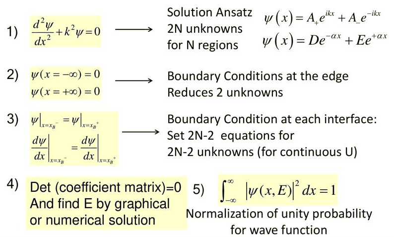
For a well of width \(W = 6\) nm and depth \(V_0 = 0.4\) eV (mass \(m = 0.067\,m_0\) everywhere), the three regions give four unknowns \((D, A_+, A_-, E')\) in \(\psi = De^{\gamma x}\) (left), \(A_+e^{ikx} + A_-e^{-ikx}\) (well), \(E'e^{-\gamma x}\) (right), with \(k = \sqrt{2mE}/\hbar\) and \(\gamma = \sqrt{2m(V_0 - E)}/\hbar\), and four matching equations at \(x = 0\) and \(x = W\). Step 4 is done here numerically: the determinant of the 4×4 matrix is evaluated on an energy grid and its sign changes are refined with a root finder.
Code
from scipy.optimize import brentq
from scipy.linalg import eigh_tridiagonal

M, W, V0 = 0.067, 6.0, 0.4


def coefficient_matrix(E):
    """Rows: ψ and ψ' continuous at x = 0 and x = W; columns: D, A+, A-, E'."""
    k, g = np.sqrt(M * E / H2M0), np.sqrt(M * (V0 - E) / H2M0)
    ep, em, eg = np.exp(1j * k * W), np.exp(-1j * k * W), np.exp(-g * W)
    return np.array(
        [[1, -1, -1, 0], [g, -1j * k, 1j * k, 0], [0, ep, em, -eg], [0, 1j * k * ep, -1j * k * em, g * eg]]
    )


def det_real(E):
    # the determinant is a complex number of constant phase (i times a real function) here
    return np.linalg.det(coefficient_matrix(E)).imag


grid = np.linspace(1e-4, V0 - 1e-4, 4000)
d = np.array([det_real(e) for e in grid])
roots = [brentq(det_real, grid[i], grid[i + 1]) for i in np.nonzero(np.sign(d[:-1]) != np.sign(d[1:]))[0]]
print("zeros of the 4×4 determinant (eV):", np.round(roots, 5))
dets = np.array([np.linalg.det(coefficient_matrix(e)) for e in grid])
print(f"largest |Re det| / |det| on the grid: {np.max(np.abs(dets.real) / np.abs(dets)):.1e}")

fig, ax = plt.subplots(figsize=(7.5, 3.6))
ax.plot(grid, d, color=style.OPEN_NEMO)
ax.axhline(0, color=style.CONTEXT, lw=0.7)
for r in roots:
    ax.axvline(r, color=style.CONTEXT, ls="--", lw=0.8)
ax.set(
    xlabel="E (eV)", ylabel="Im det (1/nm²)", ylim=(-0.06, 0.06), title="6 nm, 0.4 eV well: step 4, det = 0"
);
zeros of the 4×4 determinant (eV): [0.07823 0.28699]
largest |Re det| / |det| on the grid: 1.4e-13
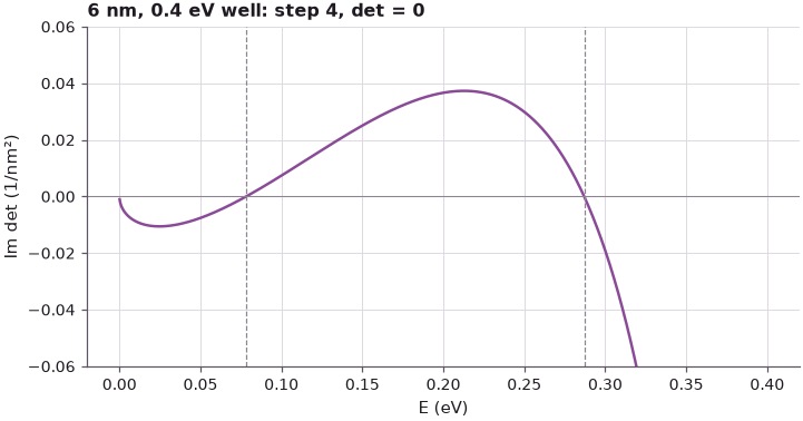
The determinant crosses zero at two energies, 0.0782 and 0.2870 eV, the two bound states of the well. (Its real part vanishes identically, to \(10^{-13}\) of its magnitude, so the imaginary part is plotted.) The same energies follow from the familiar transcendental equations \(\tan(kW/2) = \gamma/k\) and \(-\cot(kW/2) = \gamma/k\) (Section 4 checks them against the discretized Hamiltonian). The method is exact, but each new structure needs its own ansatz and its own matrix, and the size of the matrix grows with the number of regions.
2. The transfer matrix and its limits#
For open systems Lecture 6.1 replaced the determinant by the transfer matrix: one 2×2 matrix per interface, multiplied in order. Klimeck calls it "very appealing", and it works well "for simple structures like these, where you have flat bands, not too many barriers, not too thick of barriers", but "it doesn't work all that well for realistically large devices". Two reasons can be seen directly.
Flat potentials only. The plane-wave ansatz needs a constant potential in each layer. A barrier under an applied bias has a sloped top; the transfer matrix must cut it into \(n\) flat slices. Here a 5 nm, 0.3 eV barrier drops by 0.1 eV across its width (the right contact is at \(-0.1\) eV), and the sliced transfer matrix is compared with open-nemo, which simply puts the sloped potential on its grid.
Code
def interface_steps(E, widths, pots, v_left=0.0, v_right=0.0, m=M):
    """2×2 matrices S_j with [A_j, B_j] = S_j [A_j+1, B_j+1] for flat layers between two contacts."""
    k = [np.sqrt(m * (E + 1e-12j - v) / H2M0) for v in (v_left, *pots, v_right)]
    d = (0.0, *widths)
    steps = []
    for j in range(len(k) - 1):
        kj, kn = k[j], k[j + 1]
        ep, em = np.exp(1j * kj * d[j]), np.exp(-1j * kj * d[j])
        Wj = np.array([[ep, em], [1j * kj * ep, -1j * kj * em]])
        Wn = np.array([[1, 1], [1j * kn, -1j * kn]])
        steps.append(np.linalg.solve(Wj, Wn))
    return steps, k


def tmm_T(E, *args, **kw):
    out = []
    for e in np.atleast_1d(E):
        steps, k = interface_steps(e, *args, **kw)
        total = np.linalg.multi_dot(steps) if len(steps) > 1 else steps[0]
        out.append((k[-1].real / k[0].real) / abs(total[0, 0]) ** 2)
    return np.array(out)


Vb, Lb, DX = 0.1, 5.0, 0.01
gaas, bar = EM("GaAs", M, 12.9), EM("barrier", M, 12.9, conduction_band_edge=0.3)
dev = nemo.Heterostructure1D([nemo.Layer(gaas, 5.0), nemo.Layer(bar, Lb), nemo.Layer(gaas, 5.0)], spacing=DX)
u = -Vb * np.clip((dev.x - 5.0) / Lb, 0, 1)  # linear drop across the barrier, -0.1 eV in the right contact
E = np.linspace(0.01, 0.5, 120)
T_nemo = nemo.Transport(dev.hamiltonian).transmission(E, potential=u)
print(" slices n   largest |ln(T sliced TMM / T open-nemo)|")
errors = []
for n in (1, 2, 4, 8, 16, 32, 64):
    centres = (np.arange(n) + 0.5) / n * Lb
    T_tmm = tmm_T(E, [Lb / n] * n, 0.3 - Vb * centres / Lb, 0.0, -Vb)
    errors.append(np.abs(np.log(T_tmm / T_nemo)).max())
    print(f"   {n:3d}           {errors[-1]:.1e}")
 slices n   largest |ln(T sliced TMM / T open-nemo)|
     1           2.8e-02
     2           1.1e-02
     4           3.0e-03
     8           7.6e-04
    16           1.9e-04
    32           5.5e-05    64           2.1e-05
The error falls as \(1/n^2\) (a factor of four per doubling) until it reaches the discretization error of open-nemo's 0.01 nm grid, about \(2\cdot10^{-5}\), at 64 slices. Slicing works, but every non-flat region of a device (band bending, applied bias, graded alloys) multiplies the number of layers.
Loss of precision. Inside a barrier the transfer matrix carries a growing and a decaying exponential, \(e^{\pm\gamma x}\). Starting from the transmitted wave on the right and multiplying towards the left is stable: the growing exponential is the one that matters. Starting instead from the incident and reflected waves on the left, \([A, B] = [1, r]\), and propagating to the right, the wave function on the right should be the transmitted wave alone, \([t, 0]\). In floating-point arithmetic \(r\) carries a relative error of \(\epsilon \approx 10^{-16}\), and this error feeds the exponential that grows towards the right, by \(e^{2\gamma L}\).
Code
E0, V = 0.2, 0.4
g = np.sqrt(M * (V - E0) / H2M0)
print(f"E = {E0} eV, V0 = {V} eV: γ = {g:.3f} 1/nm")
print(" width (nm)   γL     |F/E| on the right, forward propagation   ε e^(2γL)")
widths = np.array([2, 5, 10, 15, 20, 25, 30])
ratios = []
for L in widths:
    steps, k = interface_steps(E0, [L], [V])
    total = steps[0] @ steps[1]
    r = total[1, 0] / total[0, 0]  # reflection amplitude B/A
    c = np.array([1.0, r])
    for S in steps:  # forward: [A_j+1, B_j+1] = S_j⁻¹ [A_j, B_j]
        c = np.linalg.solve(S, c)
    ratios.append(abs(c[1] / c[0]))
    print(
        f"   {L:4.0f}      {g * L:5.2f}            {ratios[-1]:.1e}                       "
        f"{2.2e-16 * np.exp(2 * g * L):.1e}"
    )
E = 0.2 eV, V0 = 0.4 eV: γ = 0.593 1/nm
 width (nm)   γL     |F/E| on the right, forward propagation   ε e^(2γL)
      2       1.19            4.2e-16                       2.4e-15
      5       2.97            5.9e-15                       8.3e-14
     10       5.93            7.6e-12                       3.1e-11
     15       8.90            3.5e-10                       1.2e-08
     20      11.86            4.3e-07                       4.4e-06
     25      14.83            1.1e-04                       1.7e-03
     30      17.79            1.8e-01                       6.3e-01
The amplitude of the wave incident from the right, which should be zero, grows exponentially with the barrier width and follows \(\epsilon e^{2\gamma L}\). At a width of 30 nm (\(\gamma L \approx 18\)) the spurious wave reaches 20 % of the transmitted one, and the wave function computed this way is meaningless. Lecture 6.1 showed the same loss in \(\det M\). Stable formulations (scattering matrices, or the Green's functions with open boundary conditions that open-nemo uses) avoid multiplying growing exponentials; Klimeck points to his nanoHUB course for them (Further reading).
3. Discretizing the Schrödinger equation#
The fully numerical route needs no ansatz. Space is replaced by a grid of points \(x_i = x_0 + ia\) with spacing \(a\), and the wave function by its values \(\psi_i = \psi(x_i)\). Adding the Taylor expansions of \(\psi(x_0 + a)\) and \(\psi(x_0 - a)\) cancels the odd terms:
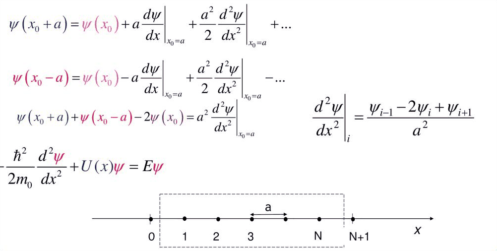
The neglected term is of order \(a^2\). For a plane wave \(e^{ikx}\) the three-point formula gives \(-(2/a^2)(1 - \cos ka)\) instead of \(-k^2\), so the kinetic energy on the grid is
a cosine band. This is the dispersion of a tight-binding chain with one s orbital per site and nearest-neighbour coupling \(-t_0\); Klimeck remarks that the natural grid spacing is therefore the atomic spacing of the crystal, which is what atomistic tight-binding models use. Below, the grid dispersion is compared with the parabola \(\hbar^2k^2/2m\) for three spacings, including one GaAs monolayer (0.2825 nm, half the cubic lattice constant).
Code
fig, (a1, a2) = plt.subplots(1, 2, figsize=(11, 4))
k = np.linspace(0, np.pi / 0.5, 400)  # wave number in 1/nm, up to the zone edge of a = 0.5 nm
a1.plot(k, H2M0 * k**2 / M, **style.series("reference"), label="parabola ħ²k²/2m")
Ekin = np.linspace(0.005, 1.0, 200)  # kinetic energy of the parabola (eV)
print(" spacing a (nm)   t0 (eV)   zone edge π/a (1/nm)   E_grid/E_parabola at E_parabola = 0.1 eV")
k01 = np.sqrt(0.1 * M / H2M0)
for a, c in zip((0.1, 0.2825, 0.5), style.sweep(3)):
    t0 = H2M0 / (M * a**2)
    a1.plot(k, 2 * t0 * (1 - np.cos(k * a)), color=c, label=f"grid, a = {a} nm")
    kE = np.sqrt(Ekin * M / H2M0)
    a2.plot(Ekin, 2 * t0 * (1 - np.cos(kE * a)) / Ekin, color=c, label=f"a = {a} nm")
    print(
        f"     {a:6.4f}       {t0:7.3f}          {np.pi / a:6.2f}                  "
        f"{2 * t0 * (1 - np.cos(k01 * a)) / 0.1:.4f}"
    )
a1.set(xlabel="k (1/nm)", ylabel="kinetic energy (eV)", ylim=(0, 10), title="dispersion, m = 0.067 m₀")
a1.legend(frameon=False, fontsize=8)
a2.set(xlabel="ħ²k²/2m (eV)", ylabel="E_grid / (ħ²k²/2m)", title="relative kinetic energy on the grid")
a2.legend(frameon=False, fontsize=8)
fig.tight_layout();
 spacing a (nm)   t0 (eV)   zone edge π/a (1/nm)   E_grid/E_parabola at E_parabola = 0.1 eV
     0.1000        56.865           31.42                  0.9999
     0.2825         7.125           11.12                  0.9988
     0.5000         2.275            6.28                  0.9963
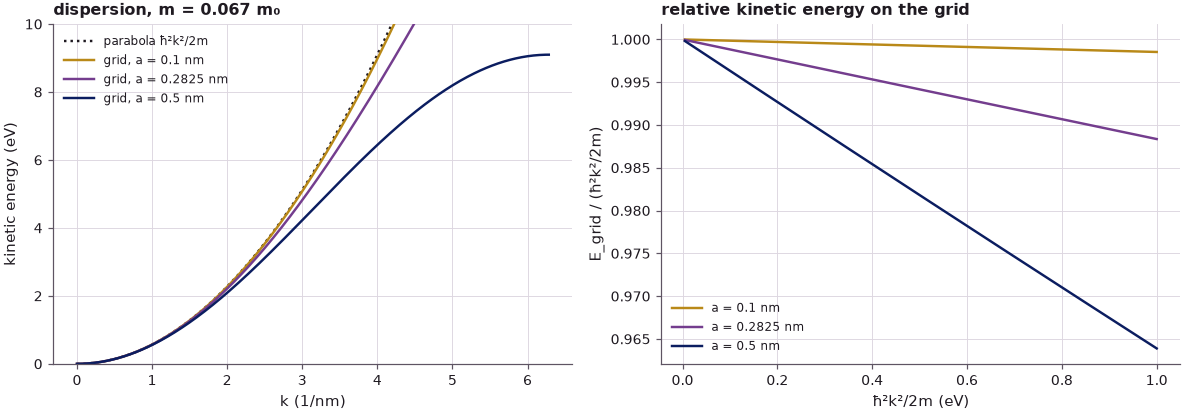
The grid underestimates the kinetic energy, by \((ka)^2/12\) to lowest order: at 0.1 eV the error is 0.01 % for \(a = 0.1\) nm, 0.12 % for one monolayer and 0.37 % for 0.5 nm. In this effective-mass model the electron energies of interest correspond to small \(ka\), and the grid is accurate. The grid cannot represent wave numbers beyond \(\pi/a\); its band ends at the zone edge with energy \(4t_0\) (9.1 eV for \(a = 0.5\) nm, the curve that bends over in the left panel).
4. The tridiagonal Hamiltonian#
Inserted into \(-\frac{\hbar^2}{2m}\psi'' + U(x)\psi = E\psi\), the three-point formula gives one equation per grid point,
with \(\psi_0 = \psi_{N+1} = 0\) for a closed system: the terms that would reach outside drop out of the first and last equations. In matrix form \(H\psi = E\psi\), with \(H\) an \(N\times N\) tridiagonal matrix: \(2t_0 + U_i\) on the diagonal and \(-t_0\) on the two neighbouring diagonals.
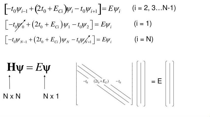
open-nemo builds the same matrix for a Heterostructure1D. The check below builds \(H\) by hand for
the 6 nm, 0.4 eV well inside 20 nm barriers and compares it element by element, then solves the
eigenvalue problem (with SciPy's tridiagonal solver, which stores only the two diagonals).
Code
def well_device(dx, barrier=20.0):
    w_mat, b_mat = EM("GaAs", M, 12.9), EM("barrier", M, 12.9, conduction_band_edge=V0)
    return nemo.Heterostructure1D(
        [nemo.Layer(b_mat, barrier), nemo.Layer(w_mat, W), nemo.Layer(b_mat, barrier)], spacing=dx
    )


dev = well_device(0.1)
t0 = H2M0 / (M * 0.1**2)
H_hand = np.diag(2 * t0 + dev.band_edge) - t0 * np.eye(dev.num_sites, k=1) - t0 * np.eye(dev.num_sites, k=-1)
H_nemo = dev.hamiltonian.sparse.dense()
print(
    f"N = {dev.num_sites} sites, t0 = {t0:.3f} eV; largest |H_hand − H_open-nemo| = "
    f"{np.abs(H_hand - H_nemo).max():.1e} eV"
)


def finite_well_levels(Wd=W, V=V0, m=M):
    f = lambda e, p: (
        np.tan(np.sqrt(m * e / H2M0) * Wd / 2) if p == 0 else -1 / np.tan(np.sqrt(m * e / H2M0) * Wd / 2)
    ) - np.sqrt((V - e) / e)
    grid = np.linspace(1e-6, V - 1e-9, 20001)
    out = []
    for p in (0, 1):
        y = f(grid, p)
        out += [
            brentq(f, grid[i], grid[i + 1], args=(p,))
            for i in np.nonzero((np.sign(y[:-1]) != np.sign(y[1:])) & (np.abs(y[:-1] - y[1:]) < 1))[0]
        ]
    return np.sort(out)


exact = finite_well_levels()
print("transcendental equations (eV):", np.round(exact, 5))
print(" spacing a (nm)   eigenvalues below V0 (eV)          largest error (meV)")
spacings = np.array([0.4, 0.2, 0.1, 0.05, 0.025])
errs = []
for a in spacings:
    h = well_device(a).hamiltonian.sparse.dense().real
    ev = eigh_tridiagonal(h.diagonal(), h.diagonal(1), select="v", select_range=(0, V0))[0]
    errs.append(np.abs(ev - exact).max())
    print(f"     {a:5.3f}        {np.array2string(ev, precision=5)}      {1e3 * errs[-1]:.4f}")
print("error ratio per halving of a:", np.round(np.array(errs[:-1]) / np.array(errs[1:]), 2))
N = 460 sites, t0 = 56.865 eV; largest |H_hand − H_open-nemo| = 0.0e+00 eV
transcendental equations (eV): [0.07823 0.28699]
 spacing a (nm)   eigenvalues below V0 (eV)          largest error (meV)
     0.400        [0.07759 0.2849 ]      2.0876
     0.200        [0.07807 0.28647]      0.5207
     0.100        [0.07819 0.28686]      0.1301
     0.050        [0.07822 0.28695]      0.0325
     0.025        [0.07823 0.28698]      0.0081
error ratio per halving of a: [4.01 4.   4.   4.  ]
The hand-built matrix and open-nemo's are identical. The eigenvalues converge to the zeros of the determinant of Section 1 and the transcendental equations, and the error falls by about a factor of four each time the spacing is halved: the \(a^2\) error of the three-point formula. Even the coarse 0.4 nm grid is within about 2 meV. The barriers are 20 nm thick so that the hard walls at the ends do not matter: the upper state decays into the barrier with \(\gamma = 0.45\) nm$^{-1}$, and with 10 nm barriers the walls would shift it by about 0.01 meV, more than the grid error at the finest spacing.
5. Closed systems are wrong for open devices#
The eigenvalue problem assumes closed boundaries, \(\psi = 0\) at both ends. For a device from which
electrons leak into contacts, this gives "just plain wrong" answers, in Klimeck's words. A double
barrier (3 nm barriers of 0.3 eV around a 5 nm well) with GaAs contacts of length \(L_c\) on each
side is solved both ways: as a closed box of total length \(2L_c + 11\) nm, and as an open system with
nemo.resonances, which attaches semi-infinite contacts through self-energies.
Code
def dbl(Lc, dx=0.05):
    g_mat, b_mat = EM("GaAs", M, 12.9), EM("barrier", M, 12.9, conduction_band_edge=0.3)
    mats, widths = (g_mat, b_mat, g_mat, b_mat, g_mat), (Lc, 3.0, 5.0, 3.0, Lc)
    return nemo.Heterostructure1D([nemo.Layer(m_, w_) for m_, w_ in zip(mats, widths)], spacing=dx)


Lcs = np.arange(8, 61, 1.0)
fig, ax = plt.subplots(figsize=(7.5, 4.5))
for Lc in Lcs:
    h = dbl(Lc).hamiltonian.sparse.dense().real
    ev = eigh_tridiagonal(h.diagonal(), h.diagonal(1), select="v", select_range=(0, 0.2))[0]
    ax.plot(np.full(ev.size, Lc), ev, ".", ms=2.5, color=style.CONTEXT)
print(" contacts Lc (nm)   closed-box eigenvalues in 0.06–0.12 eV        open system: E0 (eV)   Γ (meV)")
for Lc in (10.0, 20.0, 40.0):
    dev = dbl(Lc)
    h = dev.hamiltonian.sparse.dense().real
    ev = eigh_tridiagonal(h.diagonal(), h.diagonal(1), select="v", select_range=(0.06, 0.12))[0]
    res = nemo.resonances(dev)
    print(
        f"     {Lc:4.0f}          {np.array2string(ev, precision=4):42s}     {res['energy'][0]:.4f}     "
        f"{1e3 * res['width'][0]:.2f}"
    )
res = nemo.resonances(dbl(20.0))
ax.axhspan(
    res["energy"][0] - res["width"][0] / 2,
    res["energy"][0] + res["width"][0] / 2,
    color=style.OPEN_NEMO,
    alpha=0.25,
    lw=0,
    label="open system: resonance E0 ± Γ/2",
)
ax.set(
    xlabel="contact length Lc on each side (nm)",
    ylabel="energy (eV)",
    ylim=(0, 0.2),
    title="closed-box eigenvalues (grey) of a double barrier with contacts",
)
ax.legend(frameon=False, fontsize=8, loc="upper right");
 contacts Lc (nm)   closed-box eigenvalues in 0.06–0.12 eV        open system: E0 (eV)   Γ (meV)
       10          [0.089]                                        0.0885     4.68
       20          [0.0871 0.1089 0.1123]                         0.0885     4.78
       40          [0.0793 0.0815 0.0907 0.1171 0.1187]           0.0885     4.62
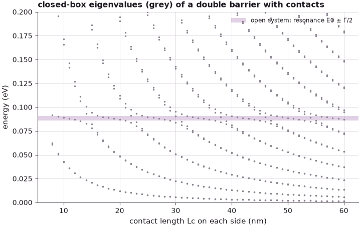
The closed box has a discrete spectrum whose energies depend on the arbitrary length of the contacts: most eigenvalues are standing waves of the contact regions, falling as \(1/L_c^2\) and appearing in nearly degenerate pairs (left and right contact). The state of the well appears as an eigenvalue only where it is not mixed with a contact state, and it is mixed more often the longer the contacts are: with 40 nm contacts there are several eigenvalues near the resonance and none of them is "the" well state. The open system gives one answer, nearly independent of \(L_c\): a resonance at 0.0885 eV with a width of 4.6 to 4.8 meV, a lifetime \(\hbar/\Gamma\) of 0.14 ps, and a continuous spectrum of contact states at every energy. These are the quantities that a transport calculation needs (Lecture 6.3), and they are invisible in the closed box.
6. Exploration: a position-dependent mass#
In a heterostructure the effective mass changes at the interfaces, for example from GaAs (\(0.067\,m_0\)) to AlGaAs (about \(0.092\,m_0\) for 30 % aluminium). Current conservation then requires \(\psi\) and \(\psi'/m\) to be continuous (BenDaniel–Duke), and the kinetic operator becomes \(-\frac{\hbar^2}{2}\frac{d}{dx}\frac{1}{m(x)}\frac{d}{dx}\). Its three-point discretization puts the mass on the bonds between sites, \(t_{i,i+1} = \hbar^2/(2m_{i+1/2}a^2)\), and keeps \(H\) symmetric; this is what open-nemo does. The naive alternative, \(-\frac{\hbar^2}{2m_i}\psi''\) with the mass on the sites, gives a non-symmetric matrix. Both are compared with the exact levels of a 6 nm well of depth 0.3 eV, whose matching condition is \(\tan(kW/2) = m_w\gamma/(m_bk)\) (even states).
Code
mw, mb, Vh = 0.067, 0.092, 0.3


def f_mass(e, p):
    k, g = np.sqrt(mw * e / H2M0), np.sqrt(mb * (Vh - e) / H2M0)
    return (np.tan(k * W / 2) if p == 0 else -1 / np.tan(k * W / 2)) - mw * g / (mb * k)


grid = np.linspace(1e-5, Vh - 1e-6, 30001)
exact = []
for p in (0, 1):
    y = f_mass(grid, p)
    exact += [
        brentq(f_mass, grid[i], grid[i + 1], args=(p,))
        for i in np.nonzero((np.sign(y[:-1]) != np.sign(y[1:])) & (np.abs(y[:-1] - y[1:]) < 1))[0]
    ]
exact = np.sort(exact)
print("exact (ψ'/m continuous):        ", np.round(exact, 5), "eV")
for a in (0.1, 0.05, 0.025):
    dev = nemo.Heterostructure1D(
        [
            nemo.Layer(EM("AlGaAs", mb, 12.9, conduction_band_edge=Vh), 20.0),
            nemo.Layer(EM("GaAs", mw, 12.9), W),
            nemo.Layer(EM("AlGaAs", mb, 12.9, conduction_band_edge=Vh), 20.0),
        ],
        spacing=a,
    )
    h = dev.hamiltonian.sparse.dense().real
    ev = eigh_tridiagonal(h.diagonal(), h.diagonal(1), select="v", select_range=(0, Vh))[0]
    m_site = np.where(np.abs(dev.x - dev.x.mean()) < W / 2, mw, mb)
    t = H2M0 / (m_site * a**2)
    H_naive = np.diag(2 * t + dev.band_edge) - np.diag(t[:-1], 1) - np.diag(t[1:], -1)
    ev_naive = np.sort(np.linalg.eigvals(H_naive).real)
    ev_naive = ev_naive[ev_naive < Vh]
    print(
        f"a = {a:5.3f} nm  mass on bonds (open-nemo):",
        np.round(ev, 5),
        f"  mass on sites (naive): {np.round(ev_naive, 5)}",
    )
exact (ψ'/m continuous):         [0.06535 0.24321] eV
a = 0.100 nm  mass on bonds (open-nemo): [0.06531 0.24313]   mass on sites (naive): [0.07715 0.25703]
a = 0.050 nm  mass on bonds (open-nemo): [0.06534 0.24319]   mass on sites (naive): [0.07718 0.25709]
a = 0.025 nm  mass on bonds (open-nemo): [0.06534 0.2432 ]   mass on sites (naive): [0.07719 0.2571 ]
The mass-on-bonds discretization converges to the exact levels; at 0.025 nm both states are within 0.01 meV. The naive discretization converges too, but to the wrong answer: 11.8 meV too high for the ground state and 14 meV for the excited state, independent of the grid. It describes a well with \(\psi'\) instead of \(\psi'/m\) continuous, which does not conserve current. Refining the grid does not fix an inconsistent discretization.
Summary#
- Closed systems can be solved analytically: ansatz, boundary conditions, a determinant set to zero, normalization. Every new geometry needs its own matrix.
- The transfer matrix solves open systems with flat layers. Sloped potentials must be sliced (error \(\propto 1/n^2\)), and propagating through thick barriers in the unstable direction amplifies round-off by \(e^{2\gamma L}\).
- On a grid of spacing \(a\) the Schrödinger equation becomes \(H\psi = E\psi\) with a tridiagonal \(H\): \(2t_0 + U_i\) on the diagonal, \(-t_0\) beside it, \(t_0 = \hbar^2/(2ma^2)\). Its error is of order \((ka)^2/12\), and its dispersion \(2t_0(1 - \cos ka)\) is that of a one-orbital tight-binding chain.
- Closed boundaries turn the continuum of the contacts into box states whose energies depend on the contact length. Devices with contacts need open boundary conditions.
- A position-dependent mass must be discretized on the bonds; the naive form converges to wrong energies.
Exercises#
- Extend
coefficient_matrixto a double well (five regions, 8×8 matrix) and find the splitting of the ground state for a 2 nm barrier between two 6 nm wells. - Use the stable (backward) propagation of Section 2 to compute the 30 nm wave function, and
compare it with open-nemo's
spectral_leftas in Lecture 6.1. - Show that the eigenvalues of the hard-wall box with \(N\) sites are exactly
\(E_n = 2t_0(1 - \cos(n\pi/(N+1)))\), and check this against
eigh_tridiagonal. - Repeat Section 5 with thicker barriers (5 nm). How long must the contacts be before the closed box shows several eigenvalues within one resonance width?
Further reading#
- Lecture 6.1: the transfer matrix method and Lecture 7.1: band structure from a periodic potential.
- Green's functions from scratch and Bound states in open devices: the open boundary conditions that replace the closed box.
- G. Klimeck, "Nanoelectronic Modeling: From Quantum Mechanics and Atoms to Realistic Devices" (2010), nanoHUB resource 8086: the course cited on slide 11.