Lecture 23.5

Theory of stress and strain — a thin layer on a substrate

In the lecture

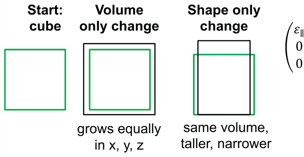
The strain of a layer splits into a volume part, $\mathrm{Tr}\,\varepsilon/3$ along every axis, and a shape part proportional to $\varepsilon_\perp - \varepsilon_\parallel$, which measures how much taller than wide the cell has become.
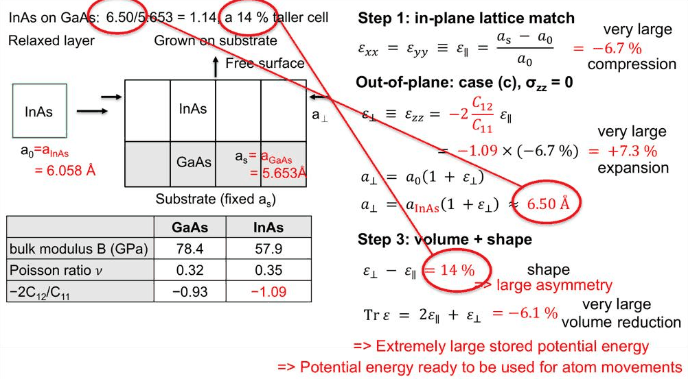
Biaxial strain in a pseudomorphic (001) layer in three steps: the layer copies the substrate spacing in-plane, its free top surface ($\sigma_{zz} = 0$) lets it bulge out, $\varepsilon_\perp = -2C_{12}/C_{11}\,\varepsilon_\parallel$, and volume and shape follow.
InAs on GaAs: $\varepsilon_\parallel = -6.7\,\%$, $\varepsilon_\perp = +7.3\,\%$, $a_\perp \approx 6.50$ Å, a volume reduction of 6.1 % and a cell 14 % taller than wide.
The stored elastic energy is very large and ready to move atoms: only about 1.7 monolayers of InAs stay flat on GaAs before quantum dots form; an InGaAs alloy stores less.

In this notebook

You split the biaxial strain of InAs on GaAs into volume and shape with kp.biaxial_strain, reproduce the slide's numbers step by step, and compare the continuum result with a finite-element layer (elasticity.Elasticity) and with the Keating valence force field, which shows where linear elasticity stops being exact at 7 % strain. You then compute the stored elastic energy per atom and per area as the film grows, for InAs and for In${0.2}$Ga${0.8}$As.

Run the notebookEvery number and figure on this page comes from it. Change it, rerun it, take it further.

Download .ipynb View on GitHub

Run it on your own machine

The notebook needs open-nemo (Python ≥ 3.10 and a C++20 compiler; BLAS/LAPACK).

git clone https://github.com/denphi/open-nemo.git && cd open-nemo
python3 -m venv .venv && source .venv/bin/activate
pip install -e ".[notebooks]"
jupyter lab From_Atoms_to_Devices/09_stress_and_strain/23_5_thin_layer_on_a_substrate.ipynb

Code12 lines · cell 1

import numpy as np
import matplotlib.pyplot as plt
import opennemo as nemo
from opennemo.visualization import style
from scipy.optimize import minimize_scalar
from opennemo.models import kp
from opennemo.models import mechanics as M
from opennemo.solvers import elasticity as E
from opennemo.solvers.poisson import Grid
from opennemo.structures.structure import Structure

style.use(notebook=True)

1. Volume and shape#

A thin layer grown on a thick substrate along [001] is strained biaxially: the substrate fixes the two in-plane directions, the top surface is free. Its strain tensor is diagonal, with the in-plane strain $\varepsilon_\parallel = \varepsilon_{xx} = \varepsilon_{yy}$ and the out-of-plane strain $\varepsilon_\perp = \varepsilon_{zz}$. It can be split into two parts with different physical meaning:

\begin{pmatrix}\varepsilon_\parallel & 0 & 0\\ 0 & \varepsilon_\parallel & 0\\ 0 & 0 & \varepsilon_\perp\end{pmatrix} = \frac{\mathrm{Tr}\,\varepsilon}{3}\begin{pmatrix}1 & 0 & 0\\ 0 & 1 & 0\\ 0 & 0 & 1\end{pmatrix} + \frac{\varepsilon_\perp - \varepsilon_\parallel}{3}\begin{pmatrix}-1 & 0 & 0\\ 0 & -1 & 0\\ 0 & 0 & 2\end{pmatrix}.

The first part is the same stretch along $x$, $y$ and $z$: a pure change of volume. The second has trace $-1 - 1 + 2 = 0$, so it changes no volume; $z$ grows while $x$ and $y$ shrink equally. It is a pure change of shape, proportional to $\varepsilon_\perp - \varepsilon_\parallel$ alone, and zero for a uniform expansion ($\varepsilon_\perp = \varepsilon_\parallel$). The aspect ratio of the strained cell makes the meaning explicit:

\frac{a_\perp}{a_\parallel} = \frac{1 + \varepsilon_\perp}{1 + \varepsilon_\parallel} \approx 1 + \varepsilon_\perp - \varepsilon_\parallel ,

so $\varepsilon_\perp - \varepsilon_\parallel$ is how much taller than wide the cell is, relative to a cube. Lecture 23.7 shows why this split matters: the volume part shifts band edges, the shape part splits the heavy and light holes.

Slide 5: a cube split into a volume change and a shape change — Slide 5. Start from a cube (left); the volume part grows it equally in $x$, $y$ and $z$; the shape part makes it taller and narrower at the same volume.

kp.biaxial_strain(material, a_substrate) returns the strain tensor of a (001) layer on a substrate of lattice constant $a_s$. For InAs on GaAs (lattice constants and elastic constants from the Vurgaftman set):

Code15 lines · cell 3

gaas, inas = kp.material("GaAs"), kp.material("InAs")
a_g, a_i = gaas.lattice_constant, inas.lattice_constant           # nm
eps = kp.biaxial_strain(inas, a_g)                                # 3x3, strain of InAs on GaAs
e_par, e_perp = eps[0, 0], eps[2, 2]
tr, shape = np.trace(eps), e_perp - e_par
volume_part = tr / 3 * np.eye(3)
shape_part = shape / 3 * np.diag([-1, -1, 2])
print("strain tensor of InAs on GaAs (%):\n", np.round(100 * eps, 2))
print(f"volume part: Tr ε / 3 = {100 * tr / 3:+.3f} % on each axis;  "
      f"shape part: (ε⊥ − ε∥)/3 = {100 * shape / 3:+.3f} % × diag(−1, −1, 2)")
print(f"volume + shape reproduces ε: {np.allclose(volume_part + shape_part, eps)}")
a_perp, a_par = a_i * (1 + e_perp), a_i * (1 + e_par)
print(f"a∥ = {10 * a_par:.4f} Å (= a_GaAs), a⊥ = {10 * a_perp:.4f} Å;  "
      f"aspect ratio a⊥/a∥ = {a_perp / a_par:.4f}"
      f",  1 + ε⊥ − ε∥ = {1 + shape:.4f}")

strain tensor of InAs on GaAs (%):
 [[-6.69  0.    0.  ]
 [ 0.   -6.69  0.  ]
 [ 0.    0.    7.27]]
volume part: Tr ε / 3 = -2.035 % on each axis;  shape part: (ε⊥ − ε∥)/3 = +4.651 % × diag(−1, −1, 2)
volume + shape reproduces ε: True
a∥ = 5.6532 Å (= a_GaAs), a⊥ = 6.4985 Å;  aspect ratio a⊥/a∥ = 1.1495,  1 + ε⊥ − ε∥ = 1.1395

The cell becomes 14.95 % taller than wide by the exact ratio, or 14.0 % by the linear estimate $1 + \varepsilon_\perp - \varepsilon_\parallel$; the two differ because 7 % is no longer a small strain. The slide's "6.50/5.653 = 1.14, a 14 % taller cell" uses the linear estimate.

2. Biaxial strain in a pseudomorphic (001) layer#

A layer is pseudomorphic when it grows atom on atom on the substrate without defects. Let its own (relaxed) lattice constant be $a_0$ and the substrate's $a_s$; the substrate is so thick that it keeps $a_s$. The derivation takes three steps.

In-plane lattice match. The layer copies the substrate spacing in the plane: $\varepsilon_{xx} = \varepsilon_{yy} \equiv \varepsilon_\parallel = (a_s - a_0)/a_0$. The strain is measured against the layer's own lattice constant, because that is what decides its forces. For $a_s < a_0$ the layer is compressed, $\varepsilon_\parallel < 0$.
Free top surface. Nothing acts on the top surface, so $\sigma_{zz} = C_{11}\varepsilon_{zz} + C_{12}(\varepsilon_{xx} + \varepsilon_{yy}) = 0$ (case (c) of Lecture 23.4), and the layer bulges out: \[\varepsilon_\perp \equiv \varepsilon_{zz} = -\frac{2C_{12}}{C_{11}}\,\varepsilon_\parallel , \qquad a_\perp = a_0(1 + \varepsilon_\perp).\] There is no shear: $\varepsilon_{xy} = \varepsilon_{yz} = \varepsilon_{xz} = 0$.
Volume and shape. \[\mathrm{Tr}\,\varepsilon = 2\varepsilon_\parallel + \varepsilon_\perp = 2\left(1 - \frac{C_{12}}{C_{11}}\right)\varepsilon_\parallel , \qquad \varepsilon_\perp - \varepsilon_\parallel = -\left(1 + \frac{2C_{12}}{C_{11}}\right)\varepsilon_\parallel .\]

Slide 7: the biaxial strain of InAs on GaAs, step by step — Slide 7. InAs ($a_0 = 6.058$ Å) on GaAs ($a_s = 5.653$ Å): $\varepsilon_\parallel = -6.7\,\%$, $\varepsilon_\perp = -1.09 \times (-6.7\,\%) = +7.3\,\%$, $a_\perp \approx 6.50$ Å; the volume shrinks by 6.1 % and the shape changes by 14 %, a very large stored potential energy.

The three steps by hand, against kp.biaxial_strain:

Code10 lines · cell 5

r12 = inas.c12 / inas.c11
step1 = (a_g - a_i) / a_i
step2 = -2 * r12 * step1
print(f"step 1: ε∥ = (a_s − a_0)/a_0 = ({10 * a_g:.3f} − {10 * a_i:.3f})/{10 * a_i:.3f} "
      f"= {100 * step1:+.2f} %")
print(f"step 2: ε⊥ = −2 C12/C11 ε∥ = {-2 * r12:.3f} × ({100 * step1:.2f} %) = {100 * step2:+.2f} %,  "
      f"a⊥ = {10 * a_i * (1 + step2):.3f} Å")
print(f"step 3: Tr ε = 2(1 − C12/C11) ε∥ = {100 * 2 * (1 - r12) * step1:+.2f} %,  "
      f"ε⊥ − ε∥ = −(1 + 2C12/C11) ε∥ = {100 * -(1 + 2 * r12) * step1:+.2f} %")
print(f"kp.biaxial_strain: ε∥ = {100 * e_par:+.2f} %, ε⊥ = {100 * e_perp:+.2f} %")

step 1: ε∥ = (a_s − a_0)/a_0 = (5.653 − 6.058)/6.058 = -6.69 %
step 2: ε⊥ = −2 C12/C11 ε∥ = -1.087 × (-6.69 %) = +7.27 %,  a⊥ = 6.499 Å
step 3: Tr ε = 2(1 − C12/C11) ε∥ = -6.11 %,  ε⊥ − ε∥ = −(1 + 2C12/C11) ε∥ = +13.95 %
kp.biaxial_strain: ε∥ = -6.69 %, ε⊥ = +7.27 %

The steps reproduce the slide: a compression of 6.69 % in the plane and an expansion of 7.27 % out of it, $a_\perp = 6.499$ Å, a volume reduction of 6.11 % and a shape change of 13.95 %. All of these are very large for a crystal; the cell is squeezed hard in the plane and stretched hard vertically.

The same layer can be computed without assuming anything about the answer. A finite-element model (as in Lecture 23.3) holds a 1 nm InAs layer on 5 nm of GaAs, gives the layer its natural lattice constant as an eigenstrain, and solves for the displacements; the top surface is free. Its local strain, measured against the InAs lattice, is printed below. An atomistic check uses the Keating valence force field: an 8-atom InAs cell is held at $\varepsilon_\parallel$ in the plane, and the out-of-plane strain that minimises its energy is found by a one-dimensional search. The cell is built at the force field's own equilibrium lattice constants (Martin's parameters in M.KEATING_PARAMETERS: $a_\mathrm{GaAs} = 5.653$ Å, $a_\mathrm{InAs} = 6.058$ Å), so that zero strain means zero force.

Code28 lines · cell 7

g = Grid(np.linspace(0, 1, 3), np.linspace(0, 1, 3), np.linspace(0, 6, 61))
C_g = E.cubic_stiffness(gaas.c11, gaas.c12, gaas.c44)
C_i = E.cubic_stiffness(inas.c11, inas.c12, inas.c44)
layer = E.Elasticity(g, C_g).cell_centers[:, 2] > 5.0
el = E.Elasticity.from_regions(g, [(None, C_g, 0.0), (layer, C_i, a_i / a_g - 1)],
                               periodic=(True, True, False))
el.fix(np.isclose(g.nodes[:, 2], 0), (0, 1, 2), 0.0)
r_fem = el.solve()
loc = r_fem.local_strain_in("biot")[layer].mean(axis=0)          # strain against the layer's own lattice
print(f"finite elements: ε∥ = {100 * loc[0, 0]:+.2f} %, ε⊥ = {100 * loc[2, 2]:+.2f} %")

tbm = nemo.structures.materials.load("klimeck2002_sp3d5s")
lat_i = nemo.structures.lattice.from_material(tbm["InAs"])
a_k = {name: M.KEATING_PARAMETERS[name][2] for name in ("GaAs", "InAs")}     # nm, VFF equilibrium
scale = a_k["InAs"] / tbm["InAs"].lattice_constant
cell_i = Structure(scale * lat_i.conventional_basis, lat_i.conventional_species, scale * lat_i.conventional,
                   lat_i.conventional_sublattice)

def keating_energy(ep, ez):                                      # eV per 8-atom cell
    s = M.strain_structure(cell_i, np.diag([ep, ep, ez]))
    return M.Keating(s).energy_and_forces(s.positions)[0]

def keating_perp(ep):
    return minimize_scalar(lambda ez: keating_energy(ep, ez), bounds=(-0.3, 0.3), method="bounded",
                           options={"xatol": 1e-9}).x

ep_vff = a_k["GaAs"] / a_k["InAs"] - 1
print(f"Keating VFF:     ε∥ = {100 * ep_vff:+.2f} %, ε⊥ = {100 * keating_perp(ep_vff):+.2f} %")

finite elements: ε∥ = -6.69 %, ε⊥ = +7.27 %
Keating VFF:     ε∥ = -6.69 %, ε⊥ = +7.17 %

The finite-element layer gives $\varepsilon_\parallel = -6.69\,\%$ and $\varepsilon_\perp = +7.27\,\%$, the continuum result, now obtained by solving the equilibrium equations with the free surface rather than by assuming $\sigma_{zz} = 0$. The force field gives $\varepsilon_\perp = +7.17\,\%$, somewhat less. (The relaxed four-monolayer film of Lecture 23.1 had 7.21 %.) The difference is not an error of either model: linear elasticity assumes the energy is quadratic in the strain, which a real bond is not at 7 %. Scanning the in-plane strain shows where the two agree:

Code24 lines · cell 9

ep_scan = np.linspace(-0.07, 0.07, 14)                           # avoids ε∥ = 0
ez_vff = np.array([keating_perp(ep) for ep in ep_scan])
c_vff = M.elastic_constants(lambda s: M.Keating(s), nemo.structures.structure.bulk(lat_i))
slope_vff = -2 * c_vff["C12"] / c_vff["C11"]
fig, (ax1, ax2) = plt.subplots(1, 2, figsize=(10, 3.8))
ax1.plot(100 * ep_scan, 100 * ez_vff, "o", color=style.OPEN_NEMO, label="Keating VFF, energy minimum")
ax1.plot(100 * ep_scan, 100 * slope_vff * ep_scan, color=style.OPEN_NEMO, lw=1,
         label=f"linear, VFF constants (−2C12/C11 = {slope_vff:.3f})")
ax1.plot(100 * ep_scan, 100 * -2 * r12 * ep_scan, "--", color=style.CONTEXT,
         label=f"linear, measured constants ({-2 * r12:.3f})")
ax1.set_xlabel("in-plane strain ε∥ (%)")
ax1.set_ylabel("out-of-plane strain ε⊥ (%)")
ax1.set_title("InAs under biaxial strain")
ax1.legend(fontsize=8)
ax2.plot(100 * ep_scan, ez_vff / ep_scan, "o-", color=style.OPEN_NEMO)
ax2.axhline(slope_vff, color=style.OPEN_NEMO, lw=1)
ax2.axhline(-2 * r12, color=style.CONTEXT, ls="--")
ax2.set_xlabel("in-plane strain ε∥ (%)")
ax2.set_ylabel("ε⊥ / ε∥")
ax2.set_title("The ratio is constant only for small strain")
plt.tight_layout()
plt.show()
print(f"VFF ε⊥/ε∥ at ε∥ = −7 %: {ez_vff[0] / ep_scan[0]:.3f};  at +7 %: {ez_vff[-1] / ep_scan[-1]:.3f};  "
      f"small-strain limit {slope_vff:.3f}")

Figure computed by the notebook with open-nemo

VFF ε⊥/ε∥ at ε∥ = −7 %: -1.068;  at +7 %: -1.243;  small-strain limit -1.148

For small strain the force field follows a straight line with its own ratio $-2C_{12}/C_{11} = -1.15$ (the Keating InAs constants of Lecture 23.1; the measured ratio is −1.09). Under compression the ratio falls to −1.068 at −7 %, under tension it rises to −1.243 at +7 %: compressed bonds stiffen, stretched bonds soften. The continuum numbers of the slide are the linear limit, accurate to a few per cent of $\varepsilon_\perp$ for InAs on GaAs; atomistic simulations of InAs dots, which reach these strains, include the anharmonic terms automatically.

3. Stored energy: why InAs films break up#

A strained crystal stores elastic energy, the work done to deform it. Per unit volume it is

w = \frac12 \sum_{ij}\sigma_{ij}\varepsilon_{ij} = \frac12\,\boldsymbol{\varepsilon}^\mathrm{T} C\,\boldsymbol{\varepsilon} \quad\text{(Voigt vectors)},

which for biaxial strain is $w = \sigma_{xx}\varepsilon_\parallel$. Klimeck compares it with a squash ball struck hard against a wall: the energy goes into the ball, which warms up. In the layer it stays stored, and it is available to move atoms as soon as the atoms find a way. Below, $w$ is converted to energy per atom (the volume per atom of the strained layer is $a_\parallel^2 a_\perp/8$) and compared with the Keating energy of the strained cell, and then to energy per area of a film of $n$ monolayers (one monolayer of a (001) zincblende film is $a_\perp/2$ thick).

Code20 lines · cell 11

eV_per_GPa_nm3 = 1e9 * 1e-27 / 1.602176634e-19                     # 1 GPa = 6.2415 eV/nm^3

def stored_energy(m, a_sub):
    e = kp.biaxial_strain(m, a_sub)
    Cm = E.cubic_stiffness(m.c11, m.c12, m.c44)
    v = E.strain_to_voigt(e)
    w = 0.5 * v @ Cm @ v * eV_per_GPa_nm3                           # eV/nm^3
    a_par, a_perp = m.lattice_constant * (1 + e[0, 0]), m.lattice_constant * (1 + e[2, 2])
    return w, w * a_par**2 * a_perp / 8, w * a_perp / 2, a_perp     # per nm^3, per atom, per nm^2 per ML

w, w_atom, w_ml, a_perp_i = stored_energy(inas, a_g)
e_vff = keating_energy(ep_vff, keating_perp(ep_vff)) / 8
print(f"InAs on GaAs: w = {w:.2f} eV/nm³ = {1000 * w_atom:.1f} meV/atom (continuum),  "
      f"Keating VFF {1000 * e_vff:.1f} meV/atom;  {w_ml:.3f} eV/nm² per monolayer")
print(f"finite elements, 1 nm layer: {r_fem.energy:.2f} eV per nm² of film")
indium = {x: stored_energy(kp.material("InGaAs", x=x), a_g) for x in (0.2, 0.5)}
for x, (wx, wa, wm, _) in indium.items():
    print(f"In{x}Ga{1 - x:.1f}As on GaAs: w = {wx:.3f} eV/nm³ = {1000 * wa:.2f} meV/atom, "
          f"{wm:.4f} eV/nm² per ML,"
          f" {w_ml / wm:.0f} × less than InAs")

InAs on GaAs: w = 2.21 eV/nm³ = 57.5 meV/atom (continuum),  Keating VFF 56.5 meV/atom;  0.719 eV/nm² per monolayer
finite elements, 1 nm layer: 2.54 eV per nm² of film
In0.2Ga0.8As on GaAs: w = 0.146 eV/nm³ = 3.38 meV/atom, 0.0424 eV/nm² per ML, 17 × less than InAs
In0.5Ga0.5As on GaAs: w = 0.770 eV/nm³ = 18.63 meV/atom, 0.2331 eV/nm² per ML, 3 × less than InAs

A layer of InAs on GaAs stores 2.21 eV per nm³, 57.5 meV per atom in the continuum model and 56.5 meV per atom with the Keating force field, a few per cent of a bond energy for every atom; every monolayer adds 0.719 eV per nm² of film. (The finite-element energy, 2.54 eV per nm² for a 1 nm layer, differs from $w \times 1$ nm because the solver measures the layer's strain against the GaAs grid, and linear elasticity depends on the reference at 7 % strain.) The stored energy grows in proportion to the film thickness:

Code14 lines · cell 13

n_ml = np.linspace(0, 12, 121)
fig, ax = plt.subplots(figsize=(7, 3.8))
ax.plot(n_ml, w_ml * n_ml, color=style.OPEN_NEMO, label="InAs on GaAs")
for (x, (_, _, wm, _)), col in zip(indium.items(), (style.REFERENCE, style.CONTEXT)):
    ax.plot(n_ml, wm * n_ml, color=col, ls="--" if x == 0.5 else "-",
            label=f"In$_{{{x}}}$Ga$_{{{1 - x:.1f}}}$As on GaAs")
ax.axvline(1.7, color="k", lw=0.8, ls=":")
ax.text(1.85, 7.5, "≈1.7 ML: InAs\nforms dots", fontsize=8)
ax.set_xlabel("film thickness (monolayers)")
ax.set_ylabel("stored elastic energy (eV/nm²)")
ax.set_title("Strain energy of a pseudomorphic film")
ax.set_ylim(0, 9.5)
ax.legend(fontsize=8)
plt.show()

In reality only about 1.7 monolayers of InAs stay flat on GaAs; a thicker film relieves its energy by clumping into islands, the self-assembled quantum dots of Lecture 23.1. (When and how a film relaxes, by islands or by misfit dislocations, depends on surface energies and growth kinetics that a bulk elastic energy does not contain; the plot only shows the driving force.) The way out is an alloy: In$x$Ga${1-x}$As has a lattice constant between those of GaAs and InAs, so it is strained less, and since the energy goes as the square of the strain (1.41 % instead of 6.69 %, Lecture 23.6), In${0.2}$Ga${0.8}$As stores 17 times less energy per monolayer than InAs (not 22 times, because the alloy is also stiffer). That is what allows pseudomorphic quantum wells of 10–20 nm, the subject of Lecture 23.6.

Summary#

Biaxial strain splits into a volume part ($\mathrm{Tr}\,\varepsilon/3$ on every axis) and a shape part $\propto \varepsilon_\perp - \varepsilon_\parallel$; the cell's aspect ratio is $a_\perp/a_\parallel \approx 1 + \varepsilon_\perp - \varepsilon_\parallel$.
For a pseudomorphic (001) layer: $\varepsilon_\parallel = (a_s - a_0)/a_0$, $\varepsilon_\perp = -2C_{12}/C_{11}\,\varepsilon_\parallel$ from the free surface, no shear.
InAs on GaAs: $\varepsilon_\parallel = -6.69\,\%$, $\varepsilon_\perp = +7.27\,\%$, $a_\perp = 6.499$ Å, Tr ε = −6.11 %, shape +13.95 % (a 14.95 % taller cell by the exact ratio). A finite-element layer gives the same numbers; the Keating force field gives $\varepsilon_\perp = 7.17\,\%$ because bonds are anharmonic at 7 % strain.
The stored energy is 57.5 meV/atom (continuum; 56.5 meV/atom Keating), 0.719 eV/nm² per monolayer; InAs films break up into dots after about 1.7 monolayers, while In${0.2}$Ga${0.8}$As stores 17 times less.

Exercises#

Compute the biaxial strain of GaAs grown on an InAs substrate (tensile). How do the volume and shape parts compare with InAs on GaAs?
Use kp.pseudomorphic_strain(inas, a_g, growth=(1, 1, 1)) for a (111) layer. Which components are nonzero, and how large are the volume and shape changes compared with (001) growth?
Repeat the Keating scan of Section 2 for GaAs (tbm["GaAs"]) and compare its ratio $\varepsilon_\perp/ \varepsilon_\parallel$ at ±7 % with InAs.
At which indium content does an In$x$Ga${1-x}$As film store as much energy in 20 nm as InAs does in 1.7 monolayers?