Lecture 23.1

Theory of stress and strain — introduction

In the lecture

Why strain matters: InAs and GaAs differ in lattice constant by about 7 %, so atoms must move when one is grown on the other, and the bands follow the atoms.
Stranski–Krastanov growth: a thin InAs wetting layer on GaAs, which clumps into self-assembled quantum dots once too much strain energy is stored.
At the nanometre scale a local 'band edge' no longer exists; what exists are confined states, easy to measure and hard to simulate.
The roadmap of Section 23: deformation (strain), internal forces (stress), material response (elastic constants), a thin layer on a substrate, and the band edges (deformation potentials).
Continuum theory against the atomistic valence force field (VFF) of NEMO 3-D: they must agree for bulk material, and differ at interfaces and on the nanometre scale.

In this notebook

You compute the lattice mismatch of common heterostructure pairs from open-nemo's parameter sets, relax a thin InAs film on a GaAs substrate atom by atom with the Keating valence force field (opennemo.models.mechanics), read the local strain off the relaxed atoms, convert it into local conduction and valence band edges with deformation potentials (opennemo.models.kp), and check that the force field reproduces the measured elastic constants of bulk GaAs and InAs, the consistency between continuum and atomistic theory that the lecture asks for.

Run the notebookEvery number and figure on this page comes from it. Change it, rerun it, take it further.

Download .ipynb View on GitHub

Run it on your own machine

The notebook needs open-nemo (Python ≥ 3.10 and a C++20 compiler; BLAS/LAPACK).

git clone https://github.com/denphi/open-nemo.git && cd open-nemo
python3 -m venv .venv && source .venv/bin/activate
pip install -e ".[notebooks]"
jupyter lab From_Atoms_to_Devices/09_stress_and_strain/23_1_stress_and_strain_introduction.ipynb

Code9 lines · cell 1

import numpy as np
import matplotlib.pyplot as plt
import opennemo as nemo
from opennemo.visualization import style
from opennemo.models import kp
from opennemo.models import mechanics as M
from opennemo.structures.structure import Structure

style.use(notebook=True)

1. Move the atoms, change the bands#

The whole section is organised around one guiding example: a thin layer of InAs (or of the alloy In$x$Ga${1-x}$As) grown on a thick GaAs substrate. The two crystals have the same zincblende structure but different lattice constants, $a_\mathrm{InAs} = 6.058$ Å and $a_\mathrm{GaAs} = 5.653$ Å. Their relative difference, the lattice mismatch

f = \frac{a_\mathrm{InAs} - a_\mathrm{GaAs}}{a_\mathrm{GaAs}} \approx 7\,\%,

is, in Klimeck's words, "a very large lattice constant difference". The substrate is so thick (a "gazillion plus one" atoms) that it does not budge. If the InAs layer is to grow on it without defects, its atoms have to line up with the substrate in the plane: the layer is compressed laterally and, in response, expands vertically. The lecturer's picture is of Lego bricks that do not quite fit, made of rubber, or gummy bears squeezed onto a rigid base. The key message is short: lattice mismatch means the atoms must move, and the bands follow the atoms.

The lattice constants below come from the k·p parameter set of Vurgaftman, Meyer and Ram-Mohan (2001), which open-nemo bundles as vurgaftman2001_kp; Si and Ge come from the tight-binding set boykin2004_sp3d5s.

Code5 lines · cell 3

gaas, inas = kp.material("GaAs"), kp.material("InAs")
a_g, a_i = gaas.lattice_constant, inas.lattice_constant           # nm, at 300 K
print(f"a(GaAs) = {10 * a_g:.4f} Å,  a(InAs) = {10 * a_i:.4f} Å")
print(f"lattice mismatch (a_InAs − a_GaAs)/a_GaAs           = {100 * (a_i - a_g) / a_g:+.2f} %")
print(f"in-plane strain of InAs on GaAs (a_GaAs − a_InAs)/a_InAs = {100 * (a_g - a_i) / a_i:+.2f} %")

a(GaAs) = 5.6532 Å,  a(InAs) = 6.0583 Å
lattice mismatch (a_InAs − a_GaAs)/a_GaAs           = +7.16 %
in-plane strain of InAs on GaAs (a_GaAs − a_InAs)/a_InAs = -6.69 %

The two numbers differ because the strain of the layer is measured against the layer's own lattice constant, $(a_\mathrm{GaAs} - a_\mathrm{InAs})/a_\mathrm{InAs}$, while the mismatch is usually quoted against the substrate. At 7 % the difference between the two conventions is already half a per cent of strain; Lecture 23.5 uses the first.

For comparison, the mismatch of a few other pairs used in heterostructures:

Code18 lines · cell 5

tb = nemo.structures.materials.load("boykin2004_sp3d5s")
pairs = [("AlAs", "GaAs"), ("GaSb", "InAs"), ("InP", "GaAs"),
         ("Ge", "Si"), ("InAs", "GaAs"), ("InSb", "GaAs")]


def lattice_constant(name):
    return tb[name].lattice_constant if name in ("Si", "Ge") else kp.material(name).lattice_constant


mismatch = [100 * (lattice_constant(a) / lattice_constant(b) - 1) for a, b in pairs]
for (a, b), f in zip(pairs, mismatch):
    print(f"{a:>4s} on {b:<4s}: {f:+6.2f} %")
fig, ax = plt.subplots(figsize=(7, 3.2))
ax.barh([f"{a} / {b}" for a, b in pairs], mismatch, color=style.OPEN_NEMO)
ax.axvline(0, color=style.CONTEXT, lw=0.8)
ax.set(xlabel="lattice mismatch (a_layer − a_substrate)/a_substrate (%)",
       title="Lattice mismatch of heterostructure pairs (300 K)")
fig.tight_layout()

AlAs on GaAs:  +0.14 %
GaSb on InAs:  +0.62 %
 InP on GaAs:  +3.83 %
  Ge on Si  :  +4.18 %
InAs on GaAs:  +7.16 %
InSb on GaAs: +14.61 %

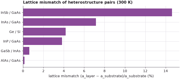
Figure computed by the notebook with open-nemo

AlAs on GaAs is almost lattice matched, which is why AlGaAs/GaAs heterostructures can be grown to any thickness. InAs on GaAs sits at the large end; only InSb on GaAs is worse.

2. Self-assembled quantum dots: what the strain does to a growing film#

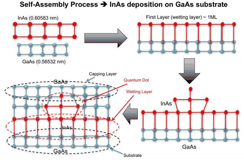
Slide 4: Stranski–Krastanov growth of InAs on GaAs — Slide 4. Stranski–Krastanov growth: the first InAs layer (the wetting layer, about one monolayer) copies the GaAs spacing in the plane; further InAs clumps into islands, which are capped with GaAs to give embedded quantum dots.

What happens if one keeps depositing InAs? The strain energy stored in the compressed film grows with its thickness, and beyond a monolayer or two the material "clumps up" to relax it: it forms small islands. Capped with GaAs, these become quantum dots that sit on a thin wetting layer, on the substrate, under a capping layer. The cartoon has a dot of four atoms; real dots contain tens of thousands of atoms and are modelled with NEMO 3-D in later sections.

Such self-assembled dots have rough, asymmetric interfaces, strain, and strain-induced (piezoelectric) polarization. This section covers the strain and its effect on the electronic structure; polarization is treated in another section.

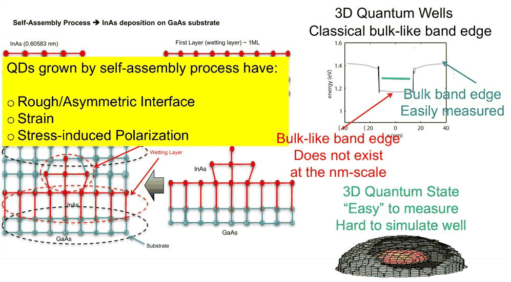
Slide 5: atom positions determine the electronic structure — Slide 5. In a thick quantum well a bulk-like band edge exists and is easily measured; at the nanometre scale a local band edge does not exist, only the confined 3-D quantum states, which are "easy" to measure and hard to simulate.

Klimeck adds a caveat that runs through the whole course. One is tempted to draw a conduction band edge through the dot, as on the slide (1.4 eV in the GaAs, lower inside). If the well were hundreds of nanometres thick, that local band edge would be a real, measurable quantity. At the nanometre scale it is not: what exists are the confined states. The band-edge pictures of this section are a continuum idealisation, useful to reason with, which atomistic models refine.

Atoms that move: a thin InAs film relaxed atom by atom#

NEMO 3-D does not compute strain with continuum theory but with an atomistic valence force field (VFF): every bond is a spring that resists stretching and bending, and the atoms move until the forces vanish. open-nemo has the same model, the Keating force field with Martin's (1970) constants (mechanics.Keating). Below, a GaAs substrate (four conventional cells, the bottom one held fixed) is covered with four monolayers of InAs (one monolayer = one cation plane plus one anion plane, $a/2$ thick). The structure is periodic in the plane with the GaAs period, so the film must match the substrate laterally; its top surface is free.

Code21 lines · cell 7

G = nemo.structures.materials.load("klimeck2002_sp3d5s")["GaAs"]     # zincblende lattice, a = 0.56533 nm
lat = nemo.structures.lattice.from_material(G)
a = G.lattice_constant
cell, basis, sub = lat.conventional, lat.conventional_basis, lat.conventional_sublattice
NX, N_SUB, N_ML = 2, 4, 4                       # in-plane cells, substrate cells, InAs monolayers
z_int = N_SUB * a                               # the interface: cations at z >= z_int become In
height = z_int + N_ML * a / 2
g = np.stack(np.meshgrid(np.arange(NX), np.arange(NX), np.arange(int(np.ceil(height / a)) + 1),
                         indexing="ij"), -1).reshape(-1, 3)
pos = ((g @ cell)[:, None, :] + basis[None]).reshape(-1, 3)
sl = np.tile(sub, len(g))
keep = pos[:, 2] < height - 1e-6
pos, sl = pos[keep], sl[keep]
species = [lat.species[s] for s in sl]
species = ["In" if (sp == "Ga" and z > z_int - 1e-6) else sp for sp, z in zip(species, pos[:, 2])]
slab = Structure(pos, species, np.array([[NX * a, 0, 0], [0, NX * a, 0]]))   # periodic in x and y only
fixed = pos[:, 2] < a - 1e-6
res = M.relax(M.Keating(slab), fixed=fixed, tol=1e-7)
x = res["positions"]
print(f"{slab.num_atoms} atoms ({species.count('In')} In), relaxed in {res['iterations']} L-BFGS steps, "
      f"converged: {res['converged']}, strain energy {res['energy']:.2f} eV")

192 atoms (32 In), relaxed in 77 L-BFGS steps, converged: True, strain energy 3.10 eV

The spacing between successive cation planes is $a/2$ in an unstrained crystal, so twice that spacing is the local vertical lattice constant $a_\perp$. In the plane every layer keeps the GaAs period.

Code19 lines · cell 9

cat = np.array([sp in ("Ga", "In") for sp in species])
z0 = np.round(pos[cat, 2], 5)
planes = np.unique(z0)
z_rel = np.array([x[cat][z0 == p, 2].mean() for p in planes])          # relaxed plane heights
is_in_plane = np.array([species[np.flatnonzero(cat)[np.argmax(z0 == p)]] == "In" for p in planes])
a_perp = 2 * np.diff(z_rel)
fig, ax = plt.subplots(figsize=(7, 3.6))
zm = 0.5 * (z_rel[1:] + z_rel[:-1])
ax.plot(zm, 10 * a_perp, "o-", color=style.OPEN_NEMO, label="Keating VFF: 2 × cation-plane spacing")
ax.axhline(10 * a_g, color=style.CONTEXT, ls=":", label="a(GaAs)")
ax.axhline(10 * a_i, color=style.REFERENCE, ls="--", label="a(InAs), unstrained")
ax.axvspan(z_int, zm.max() + 0.2, color=style.CONTEXT, alpha=0.1)
ax.text(z_int + 0.05, 10 * a_g + 0.1, "InAs film", fontsize=9)
ax.set(xlabel="height z (nm)", ylabel="local vertical lattice constant a⊥ (Å)",
       title="The atoms move: InAs on GaAs expands vertically")
ax.legend(frameon=False, fontsize=8, loc="center left")
fig.tight_layout()
print("a⊥ in the InAs film (Å):", np.round(10 * a_perp[zm > z_int], 3))
print(f"in-plane lattice constant everywhere: {10 * a_g:.4f} Å (the GaAs period)")

a⊥ in the InAs film (Å): [6.07  6.491 6.492 6.517]
in-plane lattice constant everywhere: 5.6532 Å (the GaAs period)

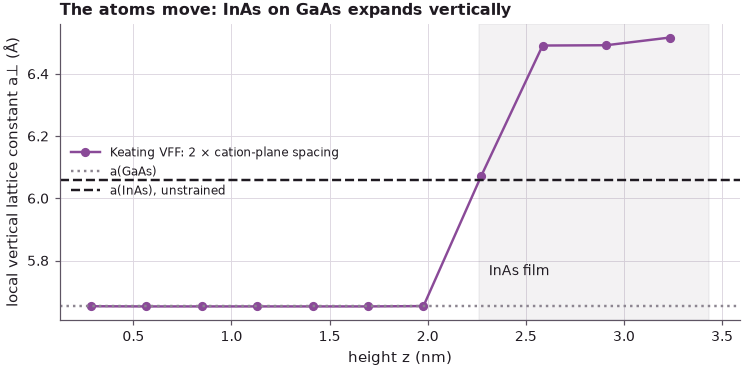
Inside the InAs film the cell is 6.49 Å tall instead of 6.058 Å (the first value, 6.07 Å, spans the interface plane and the top one, 6.52 Å, the free surface): the film is squeezed by 6.7 % in the plane and bulges out by about 7 % along the growth direction, the biaxial strain that Lecture 23.5 derives from continuum theory. The substrate below stays at the GaAs lattice constant.

The bands follow the atoms#

From the relaxed positions, mechanics.atomic_strain computes the strain tensor at every atom from its four bonds, measured against each bond's own binary (In–As bonds against InAs, Ga–As bonds against GaAs). Lecture 23.7 shows how a strain tensor shifts the band edges at Γ: the conduction band by $a_c\,\mathrm{Tr}\,\varepsilon$ and the top of the valence band by a volume term plus a heavy/light-hole splitting. kp.gamma_edge_shifts evaluates both from the 8-band k·p deformation potentials. Adding the shifts to the unstrained band edges of each material (GaAs: $E_v = -0.80$ eV, InAs: $E_v = -0.59$ eV on the common scale of the parameter set) gives local band edges, atom by atom.

Code31 lines · cell 11

loc = M.atomic_strain(slab, x, lattice_constants={("Ga", "As"): a_g, ("In", "As"): a_i})
ic = np.flatnonzero(cat & loc["valid"])                 # cations with four bonds (not the top surface)
mat = {"Ga": gaas, "In": inas}
ec, ev, ec0, ev0 = (np.zeros(len(ic)) for _ in range(4))
for sp in ("Ga", "In"):
    j = np.array([species[i] == sp for i in ic])
    dc, dv = kp.gamma_edge_shifts(mat[sp], loc["strain"][ic[j]])
    ec0[j], ev0[j] = mat[sp].conduction_band_edge, mat[sp].valence_band_offset
    ec[j], ev[j] = ec0[j] + dc, ev0[j] + dv
order = np.argsort(x[ic, 2])
zc = x[ic, 2][order]
fig, ax = plt.subplots(figsize=(7, 4))
ax.plot(zc, ec0[order], "--", color=style.CONTEXT, label="unstrained edges")
ax.plot(zc, ev0[order], "--", color=style.CONTEXT)
ax.plot(zc, ec[order], "o-", ms=3, color=style.OPEN_NEMO, label="conduction band, strained")
ax.plot(zc, ev[order], "s-", ms=3, color=style.REFERENCE, label="top valence band, strained")
ax.axvspan(z_int, zc.max() + 0.1, color=style.CONTEXT, alpha=0.1)
ax.set(xlabel="height z (nm)", ylabel="energy at Γ (eV)", title="The bands follow the atoms")
ax.legend(frameon=False, fontsize=8)
fig.tight_layout()
film = np.array([species[i] == "In" for i in ic])
eps_f = np.nanmean(loc["strain"][ic[film]], axis=0)
print("mean strain in the InAs film: ε_xx = {:+.2%}, ε_zz = {:+.2%}, Tr ε = {:+.2%}".format(
    eps_f[0, 0], eps_f[2, 2], np.trace(eps_f)))
print(f"InAs conduction band edge: {ec0[film].mean():+.3f} eV unstrained → "
      f"{ec[film].mean():+.3f} eV strained")
print(f"InAs top valence band:     {ev0[film].mean():+.3f} eV unstrained → "
      f"{ev[film].mean():+.3f} eV strained")
print(f"InAs gap at Γ: {ec0[film].mean() - ev0[film].mean():.3f} eV unstrained → "
      f"{ec[film].mean() - ev[film].mean():.3f} eV strained; unstrained conduction band offset to GaAs "
      f"{gaas.conduction_band_edge - inas.conduction_band_edge:.3f} eV")

mean strain in the InAs film: ε_xx = -6.69%, ε_zz = +7.21%, Tr ε = -6.16%
InAs conduction band edge: -0.236 eV unstrained → +0.077 eV strained
InAs top valence band:     -0.590 eV unstrained → -0.401 eV strained
InAs gap at Γ: 0.354 eV unstrained → 0.478 eV strained; unstrained conduction band offset to GaAs 0.859 eV

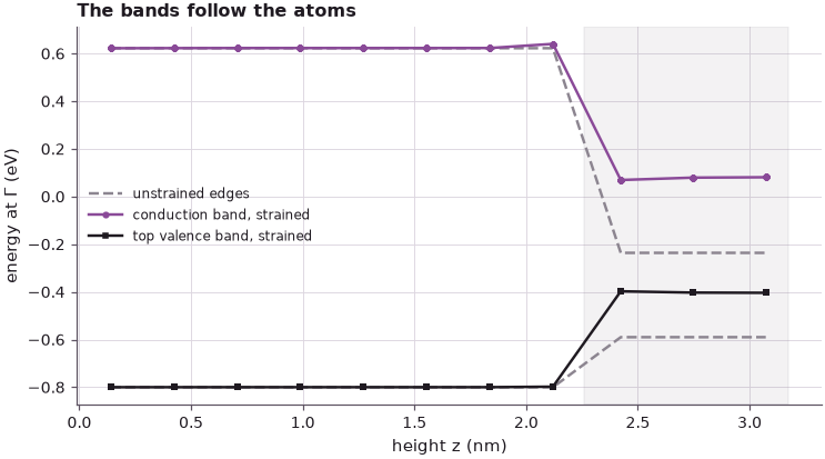
The compressed film loses 6.2 % of its volume, which pushes its conduction band up by 0.31 eV, more than a third of the 0.86 eV conduction band offset between unstrained InAs and GaAs; the top of the valence band (the heavy hole, Lecture 23.7) rises by 0.19 eV, and the gap at Γ opens from 0.354 to 0.478 eV. Strain is therefore not a small correction in this material system; it decides where the confined states sit. (The plot uses bulk deformation potentials on a film four monolayers thick; Klimeck's warning above applies, and later sections compute the confined states of such structures atomistically.)

3. The roadmap, and continuum against atomistic theory#

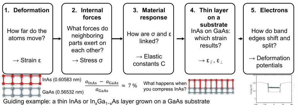
Slide 6: the five steps of Section 23 — Slide 6. The roadmap: deformation (strain ε), internal forces (stress σ), material response (elastic constants C), a thin layer on a substrate ($\varepsilon_\parallel$, $\varepsilon_\perp$), and the electrons (deformation potentials).

Steps 1 to 4 are classical continuum theory: strain, stress and the elastic constants that link them are properties of matter that have been measured for a long time, and the theory does not need atoms at all. Step 5 is quantum mechanics of the band edges and states. NEMO 3-D computes steps 1 to 4 with the atomistic valence force field instead of continuum theory, and step 5 with atomistic tight binding. The two mechanical descriptions are not independent: in the limit of bulk material they must give the same result, "if the valence force field is to represent the real material". At the nanometre scale the atomistic model adds what continuum theory cannot have: interfaces, crystal symmetry, alloy disorder.

That consistency can be checked directly. mechanics.elastic_constants strains a two-atom bulk cell, relaxes the internal coordinates and reads $C_{11}$, $C_{12}$ and $C_{44}$ off the strain energy; the measured values are those of the Vurgaftman set.

Code8 lines · cell 13

print(f"{'':6s}{'C11 (GPa)':>18s}{'C12 (GPa)':>18s}{'C44 (GPa)':>18s}{'2 C12/C11':>16s}")
print(f"{'':6s}" + "    VFF  measured" * 3 + "   VFF  meas.")
for name, km in (("GaAs", gaas), ("InAs", inas)):
    tbm = nemo.structures.materials.load("klimeck2002_sp3d5s")[name]
    prim = nemo.structures.structure.bulk(nemo.structures.lattice.from_material(tbm))
    c = M.elastic_constants(lambda s: M.Keating(s), prim)
    print(f"{name:6s}{c['C11']:7.1f}{km.c11:10.1f}{c['C12']:8.1f}{km.c12:10.1f}{c['C44']:8.1f}{km.c44:10.1f}"
          f"{2 * c['C12'] / c['C11']:8.2f}{2 * km.c12 / km.c11:7.2f}")

               C11 (GPa)         C12 (GPa)         C44 (GPa)       2 C12/C11
          VFF  measured    VFF  measured    VFF  measured   VFF  meas.
GaAs    120.4     122.1    57.0      56.6    52.0      60.0    0.95   0.93
InAs     85.3      83.3    49.0      45.3    31.4      39.6    1.15   1.09

Keating's two-parameter force field gets $C_{11}$ and $C_{12}$ within 8.3 % and $C_{44}$ (the shear constant) 13 % (GaAs) to 21 % (InAs) too low, a known limitation of the two-parameter model that richer force fields fix (see the force-field benchmarks under Further reading). For the biaxial strain of a thin layer the ratio $2C_{12}/C_{11}$ is what matters (Lecture 23.5): the VFF gives 0.95 and 1.15 against the measured 0.93 and 1.09. Linear theory with the VFF's InAs ratio would predict $\varepsilon_\perp = 1.15 \times 6.69\,\% = 7.7\,\%$; the relaxed film above has 7.2 %, because at 7 % strain the Keating energy is no longer quadratic in the strain. Close to its own bulk the force field and continuum theory agree; at large strain the atomistic model carries the anharmonic terms that linear elasticity drops.

Summary#

InAs and GaAs differ in lattice constant by 7.2 %; a layer of one on the other must deform, and the band edges move with the atoms.
Too much strain energy makes an InAs film on GaAs break up into self-assembled quantum dots (Stranski–Krastanov growth) after about a monolayer or two.
At the nanometre scale a local band edge is a continuum idealisation; the confined states are what exist.
The section builds continuum theory in five steps: strain, stress, elastic constants, the thin layer on a substrate, deformation potentials.
A Keating valence force field relaxes a thin InAs film on GaAs atom by atom: $a_\perp = 6.49$ Å, and the film's conduction band rises by 0.31 eV.
In bulk the force field must, and roughly does, reproduce the measured elastic constants.

Exercises#

Replace InAs by the alloy In${0.2}$Ga${0.8}$As in the slab (convert only one cation in five to In, at random). How much smaller are $a_\perp - a_\mathrm{GaAs}$ and the conduction band shift?
Grow the film from 2 to 8 monolayers (N_ML). Does $a_\perp$ in the middle of the film change? How does the strain energy per In atom change?
Compute the elastic constants with another force field (M.available_forcefields()), for example M.EVFF where it has GaAs parameters, and compare $C_{44}$ with the measured value.