Course/03 · Tunneling and band structure

ECE 606 Lecture 6.4

Electron tunneling — N barriers and the formation of bands

In the lecture

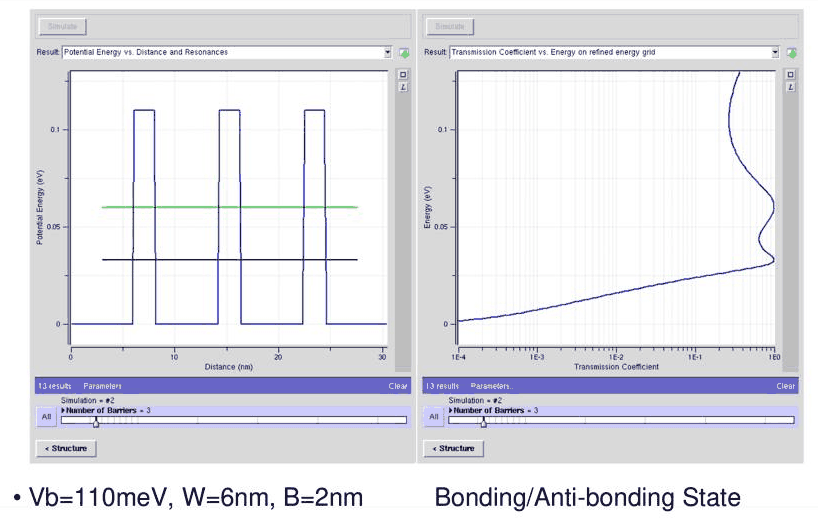
a numerical experiment with PCPBT: 110 meV barriers 2 nm wide around 6 nm wells, from one well to 49 wells
N wells give N transmission peaks: the single well state splits into N states (bonding and antibonding for two wells)
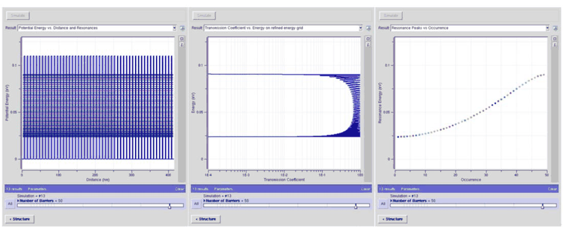
many wells form a band-pass filter, and the N states line up on a cosine-like band
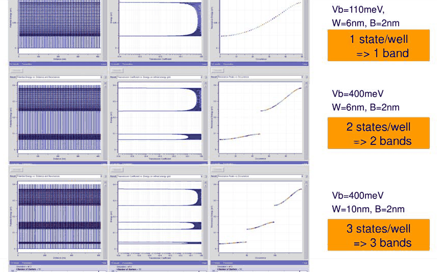
S states per well give S bands: taller barriers (400 meV) give two bands, wider wells (10 nm) three
lower bands are narrower and have a smaller slope, which means a heavier effective mass

In this notebook

repeats the lecture's experiment with open-nemo for 1 to 49 wells, counts the transmission peaks, compares the peak energies with the Bloch band of the infinite superlattice, builds the two- and three-band structures, extracts the effective mass of each band, and measures how many wells it takes to make a band.

Run the notebookEvery number and figure on this page comes from it. Change it, rerun it, take it further.

Download .ipynb View on GitHub

Run it on your own machine

The notebook needs open-nemo (Python ≥ 3.10 and a C++20 compiler; BLAS/LAPACK).

git clone https://github.com/denphi/open-nemo.git && cd open-nemo
python3 -m venv .venv && source .venv/bin/activate
pip install -e ".[notebooks]"
jupyter lab From_Atoms_to_Devices/03_tunneling_and_bandstructure/06_4_n_barriers_and_bands.ipynb

Code8 lines · cell 1

import numpy as np
import matplotlib.pyplot as plt
import opennemo as nemo
from opennemo.visualization import style

style.use(notebook=True)
H2M0 = nemo.core.units.HBAR2_2M0          # ħ²/2m₀ = 0.0381 eV nm²
EM = nemo.structures.materials.EffectiveMassMaterial

1. N wells, N transmission peaks#

The double barrier of Lecture 6.3 is one well between two barriers, and it has one transmission peak below the barrier top. The lecture adds barriers one at a time with nanoHUB's PCPBT tool, keeping each barrier \(B = 2\) nm wide and \(V_b = 110\) meV tall and each well \(W = 6\) nm wide (GaAs effective mass \(0.067\,m_0\) throughout). With \(N + 1\) barriers there are \(N\) wells, and the structure is \(N\) periods of length \(L = W + B = 8\) nm plus one closing barrier. Contacts of 10 nm GaAs at 0 eV sit on both sides.

Slide 5: two wells give two transmission peaks — Slide 5: three barriers form two wells; the single resonance of one well splits into two peaks, the analogue of a bonding and an antibonding state of a molecule.

Code39 lines · cell 3

from scipy.signal import find_peaks

M, DX, LEAD = 0.067, 0.05, 10.0


def superlattice(N, W=6.0, B=2.0, Vb=0.11, lead=LEAD, dx=DX):
    """N wells of width W between N + 1 barriers (B wide, Vb tall), GaAs contacts on both sides."""
    gaas, bar = EM("GaAs", M, 12.9), EM("barrier", M, 12.9, conduction_band_edge=Vb)
    layers = [nemo.Layer(gaas, lead)]
    for _ in range(N):
        layers += [nemo.Layer(bar, B), nemo.Layer(gaas, W)]
    layers += [nemo.Layer(bar, B), nemo.Layer(gaas, lead)]
    return nemo.Heterostructure1D(layers, spacing=dx)


def peaks(N, E, **kw):
    """Transmission and the energies of its maxima below the barrier top."""
    T = nemo.Transport(superlattice(N, **kw).hamiltonian).transmission(E)
    p = find_peaks(T)[0]
    return T, E[p][E[p] < kw.get("Vb", 0.11)]


E = np.linspace(0.0005, 0.2, 20000)
print(" wells N   transmission peaks below 110 meV   lowest (eV)   highest (eV)")
results = {}
for N in range(1, 10):
    T, ep = peaks(N, E)
    results[N] = (T, ep)
    print(f"   {N:2d}                {len(ep):2d}                        {ep[0]:.4f}        {ep[-1]:.4f}")

fig, axes = plt.subplots(1, 5, figsize=(13, 4), sharey=True)
for ax, N in zip(axes, (1, 2, 3, 5, 9)):
    T, ep = results[N]
    ax.semilogx(T, E, color=style.OPEN_NEMO, lw=0.9)
    for e in ep:
        ax.axhline(e, color=style.CONTEXT, lw=0.4, ls="--")
    ax.set(xlabel="transmission T", xlim=(1e-4, 2), title=f"{N} well{'s' if N > 1 else ''}")
axes[0].set(ylabel="energy (eV)", ylim=(0, 0.2))
fig.tight_layout();

 wells N   transmission peaks below 110 meV   lowest (eV)   highest (eV)
    1                 1                        0.0447        0.0447
    2                 2                        0.0332        0.0604
    3                 3                        0.0291        0.0694
    4                 4                        0.0272        0.0750
    5                 5                        0.0262        0.0787
    6                 6                        0.0255        0.0812
    7                 7                        0.0251        0.0830
    8                 8                        0.0249        0.0843
    9                 9                        0.0247        0.0853

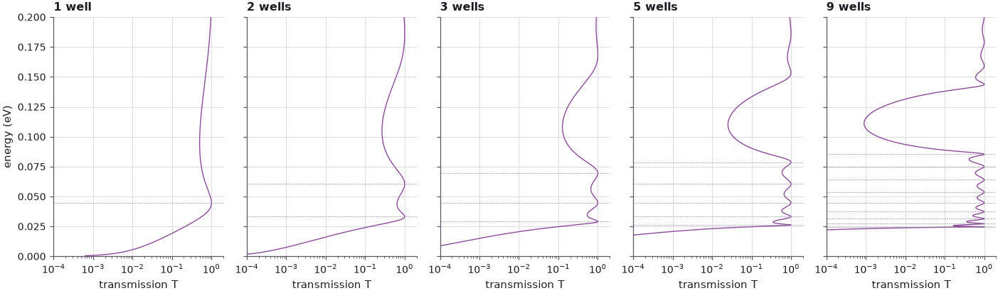
Figure computed by the notebook with open-nemo

Every added well adds one peak: one well has one resonance (at 0.045 eV), two wells have two (0.033 and 0.060 eV), and \(N\) wells have \(N\), all with \(T = 1\) for this symmetric structure. In the language of Lecture 6.3 each well alone would have a quasi-bound state at nearly the same energy; with \(N\) such wells the \(N\)-fold degenerate level splits, because the states couple through the thin barriers. The lowest peak moves down and the highest moves up as \(N\) grows, but both stay inside a fixed window (0.025 to 0.085 eV for nine wells).

2. A band-pass filter#

With 9, 19, 29 and 49 wells the peaks merge into a window of nearly perfect transmission with sharp edges, which Klimeck compares with an electrical band-pass filter. The window is the band of the infinite superlattice, the periodic repetition of one 6 nm well and one 2 nm barrier. Bloch's theorem (Lecture 7.1) gives its states: \(\psi(x + L) = e^{iqL}\psi(x)\) with \(-\pi/L \le q \le \pi/L\). open-nemo computes the band with the same discretized Hamiltonian, as a lead made of one period, with nemo.lead_bands.

Code35 lines · cell 5

def bloch_bands(W=6.0, B=2.0, Vb=0.11, dx=DX, npts=401):
    """Bands of the infinite superlattice, from one period (well + barrier) used as a lead."""
    cell = nemo.Heterostructure1D(
        [nemo.Layer(EM("GaAs", M, 12.9), W), nemo.Layer(EM("barrier", M, 12.9, conduction_band_edge=Vb), B)],
        spacing=dx,
    )
    h = cell.hamiltonian.sparse.dense().real
    V = np.zeros_like(h)
    V[-1, 0] = -H2M0 / (M * dx**2)  # the bond from the last site of one period to the next
    lead = nemo.Lead(h, V)
    bs = nemo.lead_bands(lead, npts=npts, period=W + B)
    q = bs["k"][:, 0]
    keep = q >= 0
    order = np.argsort(q[keep])
    return q[keep][order], bs["energies"][keep][order], lead


q, Eq, lead110 = bloch_bands()
bottom, top = Eq[0, 0], Eq[-1, 0]
print(
    f"Bloch band of the 6 nm / 2 nm / 110 meV superlattice: {bottom:.4f} to {top:.4f} eV "
    f"(width {1e3 * (top - bottom):.1f} meV)"
)

fig, axes = plt.subplots(1, 4, figsize=(13, 4), sharey=True)
print(" wells N   peaks   lowest (eV)   highest (eV)   mean T inside the band")
for ax, N in zip(axes, (9, 19, 29, 49)):
    T, ep = peaks(N, E)
    inside = (E > bottom) & (E < top)
    print(f"   {N:2d}      {len(ep):3d}     {ep[0]:.4f}        {ep[-1]:.4f}           {T[inside].mean():.3f}")
    ax.plot(T, E, color=style.OPEN_NEMO, lw=0.6)
    ax.axhspan(bottom, top, color=style.CONTEXT, alpha=0.15, lw=0)
    ax.set(xlabel="transmission T", xlim=(0, 1.05), title=f"{N} wells")
axes[0].set(ylabel="energy (eV)", ylim=(0, 0.12))
fig.tight_layout();

Bloch band of the 6 nm / 2 nm / 110 meV superlattice: 0.0238 to 0.0903 eV (width 66.5 meV)
 wells N   peaks   lowest (eV)   highest (eV)   mean T inside the band
    9        9     0.0247        0.0853           0.696
   19       19     0.0240        0.0889           0.698
   29       29     0.0239        0.0897           0.698
   49       49     0.0239        0.0901           0.698

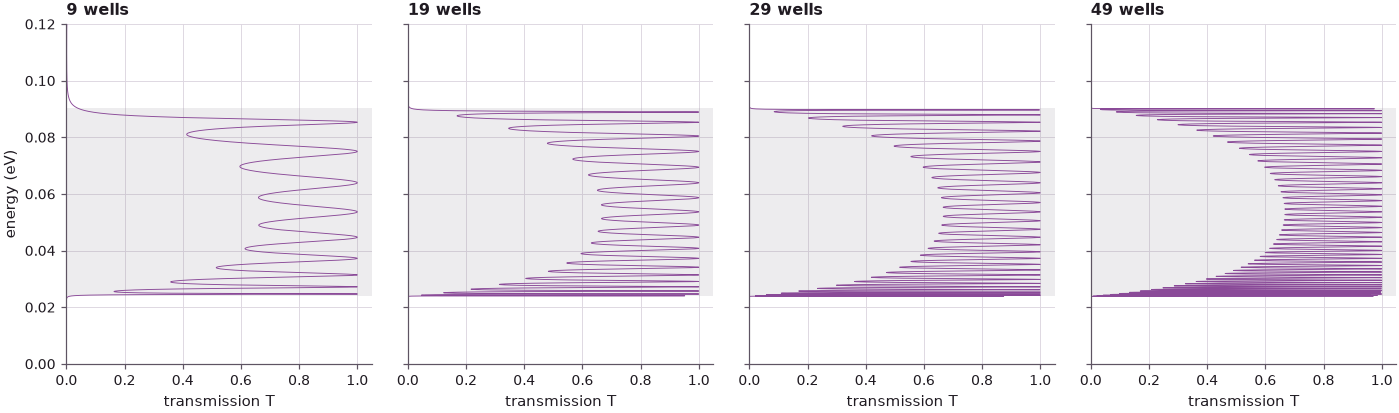
The grey band is the Bloch band of the infinite superlattice. The number of peaks still equals the number of wells (49 peaks for 49 wells), and the edges of the transmission window converge onto the Bloch band edges, 0.0238 and 0.0903 eV. Outside the band the transmission is exponentially small: these are the forbidden energies, the band gaps. As the lecture points out, the filter is not symmetric: near the lower edge the peaks are narrow and crowded, near the upper edge they are broader. The dips between the peaks do not fill in as wells are added; the transmission averaged over the band stays at 0.70 from 9 to 49 wells (Section 6 returns to this).

3. From peaks to states to a band#

The third panel of the PCPBT output plots the peak energies against their index \(j = 1 \dots N\). This relation can be made exact. The structure is \(N + 1\) identical periods (barrier plus well, the last well being the right contact), so its transfer matrix is the \((N+1)\)-th power of the matrix \(M\) of one period. Because \(\det M = 1\), the Cayley–Hamilton theorem gives

M^{n} = U_{n-1}(\xi)\,M - U_{n-2}(\xi)\,\mathbb{1}, \qquad \xi = \tfrac12\operatorname{Tr}M = \cos qL, \qquad U_n(\cos\theta) = \frac{\sin((n+1)\theta)}{\sin\theta},

where \(\xi = \cos qL\) inside a band is the Bloch condition of Lecture 7.1 and \(U_n\) are Chebyshev polynomials of the second kind. The reflection amplitude is proportional to the off-diagonal element \((M^{N+1})_{21} = U_N(\xi)M_{21}\), which vanishes when \(\sin((N+1)qL) = 0\). The transmission is therefore exactly one at

q_jL = \frac{j\pi}{N+1}, \qquad j = 1, \dots, N,

and the peaks plotted against \(q_jL/\pi = j/(N+1)\) must lie on the Bloch band \(E(q)\).

Slide 30: 49 wells, 49 peaks, 49 states — Slide 30: potential with resonance energies, transmission, and the resonance energies against their index ("occurrence") for 49 wells: a cosine-like band.

Code25 lines · cell 7

fig, ax = plt.subplots(figsize=(7.5, 4.5))
ax.plot(
    q * 8.0 / np.pi,
    Eq[:, 0],
    **style.series("reference"),
    lw=2.4,
    alpha=0.35,
    label="Bloch band of the infinite superlattice",
)
print(
    " wells N   largest |E_j − E_Bloch(q_j)| (meV)   lowest peak − band bottom (meV)   band top − "
    "highest (meV)"
)
for N, c in zip((5, 9, 19, 49), style.sweep(4)):
    _, ep = peaks(N, E)
    j = np.arange(1, len(ep) + 1)
    qj = j * np.pi / ((N + 1) * 8.0)
    dev_max = np.abs(ep - np.interp(qj, q, Eq[:, 0])).max()
    print(
        f"   {N:2d}              {1e3 * dev_max:6.2f}                          {1e3 * (ep[0] - bottom):6.2f}"
        f"                         {1e3 * (top - ep[-1]):6.2f}"
    )
    ax.plot(j / (N + 1), ep, "o", ms=3.5, color=c, label=f"{N} wells: peak j at q = jπ/((N+1)L)")
ax.set(xlabel="q L / π", ylabel="energy (eV)", xlim=(0, 1), title="transmission peaks against the Bloch band")
ax.legend(frameon=False, fontsize=8);

 wells N   largest |E_j − E_Bloch(q_j)| (meV)   lowest peak − band bottom (meV)   band top − highest (meV)
    5                0.01                            2.34                          11.63
    9                0.00                            0.84                           4.98
   19                0.00                            0.22                           1.38
   49                0.00                            0.04                           0.23

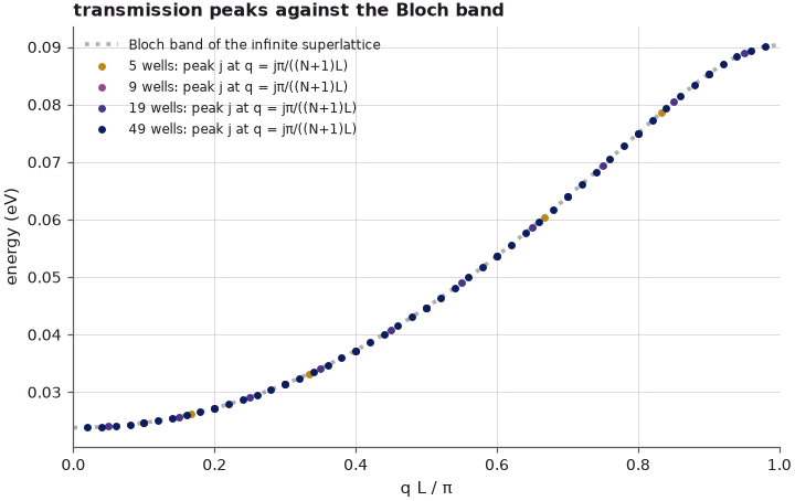
The peaks of every finite structure fall on the band of the infinite one, to 0.01 meV or better (the resolution of the energy grid), already for five wells. A finite stack does not have "almost" the band structure: its resonances sample the exact Bloch band at \(N\) discrete wave numbers. What grows with \(N\) is the sampling density. The outermost peaks sit at \(q_1 = \pi/((N+1)L)\) and \(q_N = N\pi/((N+1)L)\) and approach the band edges as \(1/(N+1)^2\), since the band is quadratic near its edges: 2.3 meV above the band bottom for five wells, 0.04 meV for 49. The band is cosine-like, flat at the bottom and at the top, and not symmetric: it is steeper above the middle than below.

The lecture adds a remark about this numerical experiment: students ask how many atoms it takes to form a band, and the answer is ambiguous, because "band structure as such is not extremely exact; it depends on the assumptions that you put in". Section 6 returns to this question.

4. S states per well give S bands#

With 110 meV barriers a 6 nm well holds one state, and the superlattice has one band. Raising the barriers to 400 meV gives each well a second state, and widening the wells to 10 nm (at 400 meV) gives a third. Each state of a single well becomes a band. The lecture shows 49 wells; 19 suffice here to see the bands, and the Bloch bands mark where they converge. The bound states of one well of the same width and depth (a finite square well) are listed for comparison.

Slide 35: one, two and three states per well give one, two and three bands — Slide 35: 110 meV with 6 nm wells (top), 400 meV with 6 nm wells (middle), 400 meV with 10 nm wells (bottom): potential, transmission, and resonance energies against their index.

Code55 lines · cell 9

from scipy.optimize import brentq


def finite_well_levels(W, V0, m=M):
    """Bound states of one square well of width W (nm) and depth V0 (eV)."""

    def f(e, parity):
        ka = np.sqrt(m * e / H2M0) * W / 2
        return (np.sqrt(e) * np.tan(ka) if parity == 0 else -np.sqrt(e) / np.tan(ka)) - np.sqrt(V0 - e)

    grid = np.linspace(1e-6, V0 - 1e-9, 20001)
    levels = []
    for parity in (0, 1):
        y = f(grid, parity)
        for i in np.nonzero((np.sign(y[:-1]) != np.sign(y[1:])) & (np.abs(y[:-1] - y[1:]) < 1))[0]:
            levels.append(brentq(f, grid[i], grid[i + 1], args=(parity,)))
    return np.sort(levels)


cases = [(6.0, 0.11), (6.0, 0.40), (10.0, 0.40)]
E4 = np.linspace(0.0005, 0.45, 30000)
fig, axes = plt.subplots(len(cases), 2, figsize=(11, 9), gridspec_kw={"width_ratios": [1, 1.2]})
bands = {}
for (W, Vb), (a1, a2) in zip(cases, axes):
    T, ep = peaks(19, E4, W=W, Vb=Vb)
    qq, EE, lead = bloch_bands(W=W, Vb=Vb)
    nb = int(np.sum(EE[0] < Vb))
    bands[(W, Vb)] = (qq, EE[:, :nb], lead)
    print(
        f"W = {W:.0f} nm, Vb = {1e3 * Vb:.0f} meV: {len(ep)} peaks with 19 wells, {nb} band(s) below the "
        "barrier top"
    )
    print("   band   bottom (eV)   top (eV)   width (meV)   single-well state (eV)")
    for n, lev in zip(range(nb), finite_well_levels(W, Vb)):
        print(
            f"    {n + 1}      {EE[:, n].min():.4f}      {EE[:, n].max():.4f}     "
            f"{1e3 * np.ptp(EE[:, n]):6.1f}"
            f"          {lev:.4f}"
        )
    a1.semilogx(T, E4, color=style.OPEN_NEMO, lw=0.5)
    a1.set(
        ylabel="energy (eV)",
        ylim=(0, 0.45),
        xlim=(1e-6, 2),
        title=f"19 wells, W = {W:.0f} nm, Vb = {1e3 * Vb:.0f} meV",
    )
    for n in range(nb):
        a1.axhspan(EE[:, n].min(), EE[:, n].max(), color=style.CONTEXT, alpha=0.2, lw=0)
        a2.plot(qq * (W + 2.0) / np.pi, EE[:, n], color=style.sweep(3)[n], lw=1.6, label=f"band {n + 1}")
    a2.axhline(Vb, color=style.CONTEXT, ls=":", lw=0.8)
    a2.set(ylabel="energy (eV)", ylim=(0, 0.45), xlim=(0, 1))
    a2.legend(frameon=False, fontsize=8, loc="upper left")
axes[-1, 0].set_xlabel("transmission T")
axes[-1, 1].set_xlabel("q L / π")
fig.tight_layout();

W = 6 nm, Vb = 110 meV: 19 peaks with 19 wells, 1 band(s) below the barrier top
   band   bottom (eV)   top (eV)   width (meV)   single-well state (eV)
    1      0.0238      0.0903       66.5          0.0468
W = 6 nm, Vb = 400 meV: 38 peaks with 19 wells, 2 band(s) below the barrier top
   band   bottom (eV)   top (eV)   width (meV)   single-well state (eV)
    1      0.0617      0.0961       34.5          0.0782
    2      0.2399      0.3822      142.4          0.2870
W = 10 nm, Vb = 400 meV: 57 peaks with 19 wells, 3 band(s) below the barrier top
   band   bottom (eV)   top (eV)   width (meV)   single-well state (eV)
    1      0.0307      0.0414       10.7          0.0364
    2      0.1215      0.1655       44.0          0.1424
    3      0.2695      0.3713      101.9          0.3037

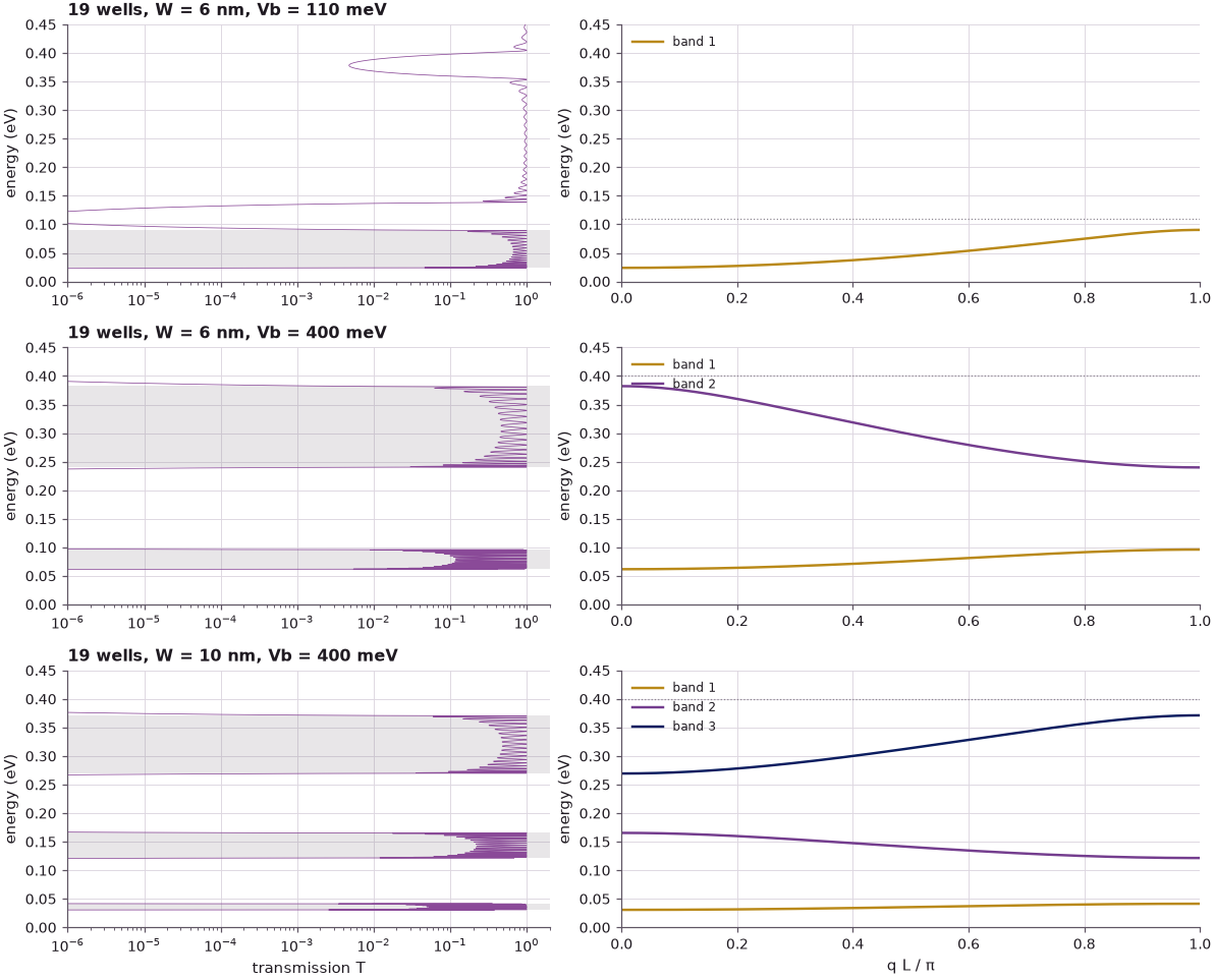
The count follows the lecture: 19 peaks per band, one band for 110 meV barriers, two bands (38 peaks) for 400 meV, three bands (57 peaks) for 400 meV and 10 nm wells. Each band contains the energy of the corresponding single-well state, and each band is separated from the next by a gap in which the transmission is exponentially small. The deepest band of the 10 nm, 400 meV superlattice is only 10.7 meV wide; the band nearest the barrier top of the same structure is 102 meV wide. A deep state is well confined, its tail in the barrier is short, and neighbouring wells couple weakly; a state near the barrier top reaches far into the barriers and couples strongly.

5. Lower bands are heavier#

Near the bottom of a band, \(E(q) \approx E_0 + \hbar^2q^2/(2m^*)\), where \(m^*\) is the effective mass of the band: the band behaves like a free electron with a different mass (Lecture 7.3 develops this). The narrower the band, the smaller its curvature, and the heavier the mass. A cosine band \(E = E_0 + 2t(1 - \cos qL)\), the result of nearest-neighbour coupling \(t\) between the wells, has width \(4t\) and \(\hbar^2/(2m^*) = tL^2\), so

\frac{m^*}{m_0} = \frac{\hbar^2/2m_0}{tL^2} = \frac{4\,(\hbar^2/2m_0)}{\Delta L^2},

with \(\Delta\) the band width. The curvature is computed from Lead.bands at small \(qL\) (dimensionless argument \(qL\) in \([-\pi, \pi]\)). For bands whose minimum is at the zone edge \(q = \pi/L\), the expansion is made there.

Code19 lines · cell 11

print(
    " W (nm)  Vb (meV)  band   minimum at   width (meV)   m*/m0 from the curvature   m*/m0 cosine "
    "4(ħ²/2m0)/(ΔL²)"
)
for (W, Vb), (qq, EE, lead) in bands.items():
    L = W + 2.0
    for n in range(EE.shape[1]):
        q0 = 0.0 if EE[0, n] < EE[-1, n] else np.pi  # where the band has its minimum
        dq = 0.02
        e0 = lead.bands(np.array([q0]))[0][n]
        e1 = lead.bands(np.array([q0 - dq]))[0][n]
        mass = H2M0 * (dq / L) ** 2 / (e1 - e0)
        width = np.ptp(EE[:, n])
        where = "q = 0  " if q0 == 0 else "q = π/L"
        print(
            f"  {W:4.0f}     {1e3 * Vb:4.0f}      {n + 1}     {where}      {1e3 * width:6.1f}            "
            f" {mass:6.3f}"
            f"                     {4 * H2M0 / (width * L**2):6.3f}"
        )

 W (nm)  Vb (meV)  band   minimum at   width (meV)   m*/m0 from the curvature   m*/m0 cosine 4(ħ²/2m0)/(ΔL²)
     6      110      1     q = 0          66.5              0.070                      0.036
     6      400      1     q = 0          34.5              0.095                      0.069
     6      400      2     q = π/L       142.4              0.021                      0.017
    10      400      1     q = 0          10.7              0.123                      0.099
    10      400      2     q = π/L        44.0              0.029                      0.024
    10      400      3     q = 0         101.9              0.011                      0.010

Within each structure the mass grows as the band goes down: in the 10 nm, 400 meV superlattice the lowest band (\(0.123\,m_0\)) is eleven times heavier than the highest (\(0.011\,m_0\)). This is the lecture's last observation: lower bands have smaller slopes and therefore heavier masses. The bands near the barrier top are even lighter than the GaAs mass \(0.067\,m_0\) of the material, a reminder that \(m^*\) is a property of the band, not of the material alone. The cosine estimate from the band width has the right trend but is 10 to 50 % too light, because the real bands are flatter at the bottom than a cosine of the same width (the 110 meV band is the extreme case, a factor of two).

The second band of each structure is upside down, with its minimum at the zone edge \(q = \pi/L\) and its maximum at \(q = 0\): the bands alternate, like bonding and antibonding combinations of the single-well states.

6. Exploration: how many wells make a band?#

Klimeck's answer to the question of how many atoms it takes to make a band is that it depends on what one asks of the band. Section 3 showed that the energies are exact Bloch-band energies for any \(N\). Two transport measures, computed for the 110 meV structure as a function of the number of wells: the transmission averaged over the Bloch band (how good the pass band is) and the largest transmission in the gap 5 to 15 meV above the band top (how good the stop band is).

Code17 lines · cell 13

Ns = np.array([1, 2, 3, 4, 6, 9, 14, 19, 29, 39, 49])
inside = (E > bottom) & (E < top)
gap = (E > top + 0.005) & (E < top + 0.015)
pass_T, stop_T = [], []
for N in Ns:
    T = nemo.Transport(superlattice(N).hamiltonian).transmission(E)
    pass_T.append(T[inside].mean())
    stop_T.append(T[gap].max())
print(" wells N   mean T in the band   max T in the gap")
for N, a, b in zip(Ns, pass_T, stop_T):
    print(f"   {N:2d}           {a:.3f}            {b:.1e}")
fig, (a1, a2) = plt.subplots(1, 2, figsize=(11, 3.8))
a1.plot(Ns, pass_T, "o-", color=style.OPEN_NEMO, ms=4)
a1.set(xlabel="number of wells N", ylabel="mean T inside the Bloch band", title="pass band")
a2.semilogy(Ns, stop_T, "o-", color=style.OPEN_NEMO, ms=4)
a2.set(xlabel="number of wells N", ylabel="max T 5–15 meV above the band", title="stop band")
fig.tight_layout();

 wells N   mean T in the band   max T in the gap
    1           0.659            5.1e-01
    2           0.667            2.8e-01
    3           0.677            1.6e-01
    4           0.684            9.0e-02
    6           0.692            2.9e-02
    9           0.696            5.6e-03
   14           0.697            3.6e-04
   19           0.698            2.4e-05
   29           0.698            1.0e-07
   39           0.698            4.2e-10
   49           0.698            1.8e-12

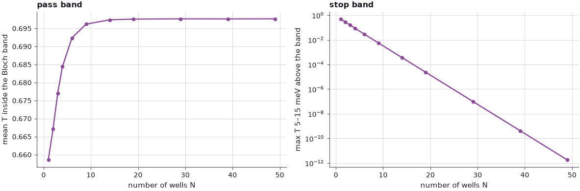
The two measures behave very differently. The stop band improves exponentially: every added period multiplies the largest transmission in the gap by a roughly constant factor (about 1.7 from 19 to 49 wells, from \(2\cdot10^{-5}\) to \(2\cdot10^{-12}\)), because in the gap the Bloch wave number is complex and the wave decays from period to period. The pass band hardly changes: the mean transmission inside the band is 0.66 for one well and 0.70 for 49. The peaks multiply, but the dips between them stay as deep, because the dips are set by the mismatch between the plane waves of the contacts and the Bloch waves of the superlattice, a property of each period and not of their number. A band in the sense of a range of perfect transmission never forms in this open structure; what forms is a range of energies that is allowed, sharply separated from ranges that are forbidden. The next lectures take the limit of the infinite periodic structure directly with Bloch's theorem.

Summary#

\(N\) coupled wells have \(N\) transmission peaks: the degenerate single-well level splits into \(N\) states (bonding and antibonding for \(N = 2\)).
Many wells make a band-pass filter. For \(N + 1\) identical barriers the peaks lie exactly on the Bloch band of the infinite superlattice, at \(q_j = j\pi/((N+1)L)\); more wells sample the band more densely.
Outside the bands the transmission is exponentially small and gets smaller with every period: band gaps.
\(S\) states per well give \(S\) bands; deeper states give narrower bands.
Narrow bands have small curvature and heavy effective masses, \(m^*/m_0 \approx 4(\hbar^2/2m_0)/(\Delta L^2)\) for a cosine band of width \(\Delta\).

Exercises#

Increase the barrier width of the 110 meV superlattice from 2 nm to 4 nm. Predict the change of the band width and of the effective mass, then compute both.
Make one barrier of the 19-well structure 3 nm instead of 2 nm. What happens to the peaks of the pass band?
Compute the lower envelope of the dips between the peaks of the 49-well structure and compare it with \(1/(1 + |M_{21}|^2/\sin^2 qL)\), using the transfer matrix \(M\) of one period from Lecture 6.1 (hint: \(|U_N(\cos qL)| \le 1/|\sin qL|\)).
Use superlattice(N) with 400 meV barriers and \(N = 2\): compute the splitting of the lower and of the upper single-well state, and compare the ratio of the two splittings with the ratio of the two band widths of Section 4.