Lecture 11.2

RTDs with realistic doping profiles

In the lecture

why real RTDs keep the dopants 20–100 nm away from the barriers (undoped spacers against ionized-impurity scattering), and what that does to the electrostatics
the Thomas–Fermi (semiclassical) electron density and the Poisson equation: the RTD floats up above the Fermi levels in equilibrium
under bias: charge accumulation in the emitter, depletion in the collector, a triangular potential well (notch) in front of the first barrier and an unphysical classical charge spike
the quasi-bound emitter states E1 and E2 in that notch, and the extra I–V peaks that appear when the central resonance C1 lines up with them
traces of the critical energies against bias, and resonance widths: E1 narrows exponentially with bias, C1 hardly changes; the narrower of the two states limits the current

In this notebook

builds an RTD with $10^{18}$ cm$^{-3}$ contacts and 50 nm undoped spacers, solves the Thomas–Fermi/Poisson problem with nemo.thomas_fermi_iv (ballistic current, Fermi level dropping linearly across the device), plots band profiles and charge at 0 and 0.32 V, finds the emitter notch states with nemo.resonances, computes the multi-peak I–V curve and the current spectrum at its peaks, traces C1, E1, E2 and the emitter band edges against bias with their widths, and varies the spacer length.

Run the notebookEvery number and figure on this page comes from it. Change it, rerun it, take it further.

Download .ipynb View on GitHub

Run it on your own machine

The notebook needs open-nemo (Python ≥ 3.10 and a C++20 compiler; BLAS/LAPACK).

git clone https://github.com/denphi/open-nemo.git && cd open-nemo
python3 -m venv .venv && source .venv/bin/activate
pip install -e ".[notebooks]"
jupyter lab From_Atoms_to_Devices/06_resonant_tunneling_diodes/11_2_rtds_with_realistic_doping.ipynb

Code8 lines · cell 1

import numpy as np
import matplotlib.pyplot as plt
import opennemo as nemo
from opennemo.visualization import style

style.use(notebook=True)
H2M0 = nemo.core.units.HBAR2_2M0          # ħ²/2m₀ = 0.0381 eV nm²
EM = nemo.structures.materials.EffectiveMassMaterial

1. From linear drops to a realistic doping profile#

Lecture 11.1 assumed that the potential is flat in both contacts and drops linearly across barriers and well. The resonances then fall linearly with bias, act as bandpass filters pulled through the electron supply, and the current turns on when a resonance enters the thermal sea of electrons and off when it passes under the emitter conduction band edge. This lecture asks what the electrostatic potential of a real RTD looks like.

A useful RTD needs high current densities, so the contacts are doped heavily, typically to $10^{18}$ cm$^{-3}$. If the dopants come close to the double barrier, scattering by the ionized impurities spoils the resonance. Real devices therefore have undoped spacers, 20 to 100 nm long, between the heavily doped contacts and the barriers; the spacers contain only the unintentional background doping, of order $10^{15}$ cm$^{-3}$.

2. Thomas–Fermi charge and the Poisson equation#

Electrons diffuse from the doped contacts into the spacers, where there are more electrons than donors. The negative net charge raises the electrostatic potential energy until the diffusion is balanced. To compute this the lecture uses the Thomas–Fermi (semiclassical) density: at every point the electrons fill a local bulk conduction band whose edge is $E_c(x)$,

n(x) = N_c\,\mathcal{F}_{1/2}\!\left(\frac{E_F(x) - E_c(x)}{k_BT}\right) \;\approx\; N_c\, e^{(E_F(x)-E_c(x))/k_BT},

where $N_c = 2\,(m^* k_BT/2\pi\hbar^2)^{3/2}$ is the effective density of states of the conduction band, $\mathcal{F}_{1/2}$ the Fermi–Dirac integral and the exponential its non-degenerate (Boltzmann) limit. The potential $V(x)$ follows from the Poisson equation,

\frac{d}{dx}\left(\varepsilon(x)\frac{dV}{dx}\right) = -q\,[N_D(x) - n(x)],

with $N_D$ the donor density and $\varepsilon$ the permittivity, and $E_c(x) = E_{c,0}(x) - qV(x)$ where $E_{c,0}$ is the band offset profile. Density and potential depend on each other, and the pair of equations is iterated to self-consistency. The calculation is very fast, which is why it is the first step; its limitations are the subject of the next lectures.

In equilibrium the Fermi level $E_F$ is constant. Under bias the lecture assumes that the barriers isolate the emitter and collector well, so the Fermi levels are nearly flat in both, and that the quasi-Fermi level drops linearly across the device in between, a pure assumption made to have a classical charge everywhere. nemo.thomas_fermi_iv implements exactly this model (the Ptype = ThomasFermi model of NEMO-1D); with charge="all" the semiclassical density is put on every site, also in the barriers and the well, and relaxation=None computes the current ballistically from the transmission through the self-consistent potential.

The device below has 30 nm GaAs contacts doped to $10^{18}$ cm$^{-3}$, 50 nm spacers doped to $10^{15}$ cm$^{-3}$, and a double barrier of 4 nm Al${0.3}$Ga${0.7}$As, a 5 nm GaAs well and another 4 nm barrier. The barriers and well are thinner than in lecture 11.1 so that the ground-state width, about 0.4 meV, is close to the one in the lecture's example.

Code32 lines · cell 4

x_al = 0.3
gaas = EM("GaAs", 0.067, 12.9, conduction_band_edge=0.0)
algaas = EM("Al0.3Ga0.7As", 0.067 + 0.083 * x_al, 12.9 - 2.84 * x_al, conduction_band_edge=0.324)


def make_rtd(spacer=50.0, barrier=4.0, well=5.0, contact=30.0):
    layers = [
        nemo.Layer(gaas, contact, donors=1e18, name="emitter contact"),
        nemo.Layer(gaas, spacer, donors=1e15, name="emitter spacer"),
        nemo.Layer(algaas, barrier, name="barrier"),
        nemo.Layer(gaas, well, name="well"),
        nemo.Layer(algaas, barrier, name="barrier"),
        nemo.Layer(gaas, spacer, donors=1e15, name="collector spacer"),
        nemo.Layer(gaas, contact, donors=1e18, name="collector contact"),
    ]
    return nemo.Heterostructure1D(layers, spacing=0.25, terminal_layers=(2, 2))


rtd = make_rtd()
x = rtd.x
XB1 = 30.0 + 50.0  # position of the first barrier (nm)
emitter = x < XB1
T = 300
V = np.round(np.arange(0.0, 0.7001, 0.005), 3)
tf = nemo.thomas_fermi_iv(rtd, V, T, charge="all", relaxation=None)
J = tf["current_density"]
Ec = rtd.band_edge[None, :] + tf["potential"]  # conduction band edge at every bias (eV)
EF = float(np.atleast_1d(tf["mu_left"])[0])
print(
    f"{rtd.num_sites} sites, {len(V)} biases; emitter Fermi level {1e3 * EF:.1f} meV above the contact "
    "band edge"
)

692 sites, 141 biases; emitter Fermi level 41.9 meV above the contact band edge

Code26 lines · cell 5

i0, i32 = 0, int(np.argmin(abs(V - 0.32)))
fig, axes = plt.subplots(2, 2, figsize=(10, 6.4), sharex=True)
for col, i in zip(axes.T, (i0, i32)):
    # the band edge is the structure, not a compared series: a solid dark outline, and the
    # quasi-Fermi level dashed over it
    col[0].plot(x, Ec[i], color=style.REFERENCE, lw=1.2, label="conduction band edge")
    col[0].plot(x, tf["fermi_level"][i], **style.series(variant=1, lw=1.2), label="quasi-Fermi level")
    col[0].set(ylabel="Energy (eV)", title=f"{V[i]:.2f} V", ylim=(-0.45, 0.45))
    col[1].semilogy(x, tf["electron_density"][i], **style.series(), label="electrons (Thomas–Fermi)")
    col[1].semilogy(x, rtd.donors, **style.series("nemo-family"), label="donors")
    col[1].set(xlabel="Position (nm)", ylabel="Density (cm$^{-3}$)", ylim=(1e14, 3e18))
axes[0, 0].legend(fontsize=8)
axes[1, 0].legend(fontsize=8, loc="lower left")
fig.tight_layout()

ec0 = Ec[i0]
print(
    f"0 V: spacer band edge rises to {1e3 * ec0[emitter].max():.0f} meV, "
    f"{1e3 * (ec0[emitter].max() - EF):.0f} meV above the Fermi level"
)
for i in (i0, i32):
    n = tf["electron_density"][i]
    print(
        f"{V[i]:.2f} V: n just before the first barrier {n[emitter][-1]:.2g} cm^-3, "
        f"lowest n in the emitter spacer {n[emitter].min():.2g} cm^-3"
    )

0 V: spacer band edge rises to 114 meV, 72 meV above the Fermi level
0.00 V: n just before the first barrier 2.6e+16 cm^-3, lowest n in the emitter spacer 2.6e+16 cm^-3
0.32 V: n just before the first barrier 3.5e+17 cm^-3, lowest n in the emitter spacer 8.1e+16 cm^-3

Figure computed by the notebook with open-nemo

Slide 9. (a, c) Conduction band and Fermi levels at 0 V and 0.32 V; (b, d) electron density and doping on a log scale. At 0.32 V a triangular well with the emitter state E1 forms in front of the first barrier, electrons accumulate in the emitter and the collector spacer is depleted.

At zero bias the electrons that spill out of the contacts raise the spacers' band edge into a broad hump, and the whole double barrier floats up with it, well above the Fermi levels. Under 0.32 V three things happen, exactly as on the slide:

Accumulation in the emitter. The electron density in front of the first barrier rises above the contact doping. This charge resists the pull of the collector: the emitter potential barely moves.
Depletion in the collector. The collector spacer has almost no free charge, so the potential drops nearly linearly there, and most of the applied voltage is dropped on the collector side.
A triangular notch. Between the emitter hump and the first barrier the band edge forms a triangular potential well. Classically it fills with electrons, which shows up as a sharp density spike against the barrier. The lecturer points out that this spike is not physical: the electron wave functions vanish at the barrier and the notch holds discrete quantum states, which would smooth it. The model also assumes a Fermi level inside the RTD, which does not really exist.

3. Quantum states in the emitter notch#

A triangular well binds quasi-bound states. The emitter notch therefore has its own resonances E1, E2, ..., coupled weakly to the emitter contact through the hump and to the central well through the first barrier. nemo.resonances finds them when its confinement region is extended into the emitter (confinement_region=(-160, 0) lets the search region start 160 sites, 40 nm, before the first barrier). The function below sorts the states at one bias into the central resonance C1, located in the well, and the notch states, located in the emitter below its top.

Code27 lines · cell 9

def states(i):
    """C1 and the emitter notch states at bias index i: dict of (energy, width) arrays."""
    ec = Ec[i]
    top, bottom = ec[emitter].max(), ec[emitter][-1]
    r = nemo.resonances(
        rtd, potential=tf["potential"][i], confinement_region=(-160, 0), emin=bottom - 0.005, emax=0.3
    )
    e, g, x0 = r["energy"], r["width"], r["x0"]
    narrow = np.flatnonzero((g < 5e-3) & (x0 > XB1 - 30))
    c1 = narrow[np.argmax(x0[narrow])]  # the narrow state farthest to the right is the central one
    notch = np.flatnonzero((e < top + 0.003) & (x0 < XB1 + 6) & (np.arange(len(e)) != c1))
    sharp = notch[g[notch] < 5e-3]  # E1: the lowest sharp notch state
    e1 = sharp[np.argmin(e[sharp])] if len(sharp) else None
    rest = [k for k in notch[np.argsort(e[notch])] if k != e1]
    picked = ([e1] if e1 is not None else []) + rest[:1]
    central = np.arange(len(e)) == c1
    sel = np.array(picked, dtype=int)
    return dict(top=top, bottom=bottom, C=(e[central], g[central]), E=(e[sel], g[sel]), has_E1=e1 is not None)


for v in (0.32, 0.42):
    s = states(int(np.argmin(abs(V - v))))
    print(
        f"{v:.2f} V: emitter top {1e3 * s['top']:.1f} meV, bottom {1e3 * s['bottom']:.1f} meV; "
        f"C1 {1e3 * s['C'][0][0]:.1f} meV; notch states "
        + ", ".join(f"E{k + 1} {1e3 * e:.1f} meV" for k, e in enumerate(s["E"][0]))
    )

0.32 V: emitter top 83.6 meV, bottom 40.6 meV; C1 91.3 meV; notch states E1 76.3 meV, E2 83.6 meV
0.42 V: emitter top 81.6 meV, bottom 27.8 meV; C1 68.4 meV; notch states E1 70.1 meV, E2 83.4 meV

Slide 10: transmission and current density when C1 is aligned with E2 (0.32 V) and with E1 (0.42 V) — Slide 10. Band diagram, transmission and current density at 0.32 V, where C1 lines up with the emitter state E2, and at 0.42 V, where it lines up with E1. The green running integral shows that at 0.32 V practically all the current flows through the C1–E2 alignment and at 0.42 V about 92% through C1–E1.

4. The current–voltage characteristic: the central resonance probes the emitter#

The ballistic current density of the Thomas–Fermi potential has more than one peak. The central resonance is pulled through an emitter that is no longer a flat sea of electrons but contains discrete notch states; every time C1 lines up with one of them, it finds a strong source of electrons.

Code18 lines · cell 12

i_pk = int(np.argmax(J))
win = (V > V[i_pk] + 0.05) & (V < 0.5)
i_2 = int(np.flatnonzero(win)[np.argmax(J[win])])
i_v = i_2 + int(np.argmin(J[i_2 : i_2 + 30]))
print(
    f"main peak {J[i_pk]:.0f} A/cm^2 at {V[i_pk]:.3f} V; second peak {J[i_2]:.0f} A/cm^2 at {V[i_2]:.3f} V; "
    f"valley {J[i_v]:.0f} A/cm^2 at {V[i_v]:.3f} V"
)

fig, ax = plt.subplots(figsize=(6, 3.6))
ax.plot(V, J, color=style.OPEN_NEMO, lw=2)
for i in (i_pk, i_2):
    ax.axvline(V[i], color="C3", ls="--", lw=1)
ax.set(
    xlabel="Bias (V)",
    ylabel="Current density (A/cm²)",
    title="Thomas–Fermi potential, ballistic current, 300 K",
);

main peak 2403 A/cm^2 at 0.320 V; second peak 609 A/cm^2 at 0.415 V; valley 74 A/cm^2 at 0.445 V

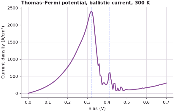
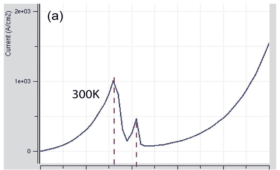
Slide 11: the computed I–V curve with two peaks — Slide 11. The lecture's I–V characteristic at 300 K (0 to 1 V): a main peak, a second, smaller peak, then a valley and a rising background.

The two curves look alike: a main peak near 0.32 V, and a second, sharp peak about 0.1 V later, followed by a valley. Between them the computed curve has a few narrow wiggles where C1 passes higher notch states.

To see which states carry the current at the two peaks, the current spectrum $J(E)$ is computed with nemo.Transport on an energy grid refined around all resonances (some are only microelectronvolts wide), and its running integral is split at the midpoints between the resonance energies.

Code38 lines · cell 15

tr = nemo.Transport(rtd.hamiltonian)


def current_spectrum(i):
    u = tf["potential"][i]
    mu_l, mu_r = EF, EF - V[i]
    r = nemo.resonances(
        rtd, potential=u, confinement_region=(-160, 0), emin=Ec[i][emitter][-1] - 0.005, emax=0.35
    )
    seeds = [e + max(w, 1e-7) * np.linspace(-15, 15, 151) for e, w in zip(r["energy"], r["width"])]
    E = np.unique(np.concatenate([np.linspace(1e-5, mu_l + 15 * 8.617e-5 * T, 3000)] + seeds))
    E = E[(E > 0) & (E < mu_l + 15 * 8.617e-5 * T)]
    t = tr.transmission(E, potential=u)
    Je = rtd.current_spectrum(E, t, mu_l, mu_r, T)
    return E, t, Je, rtd.current_density(E, t, mu_l, mu_r, T)


fig, axes = plt.subplots(1, 3, figsize=(11, 3.8), sharey=True, gridspec_kw=dict(width_ratios=[1.3, 1, 1]))
for i, c in ((i_pk, style.OPEN_NEMO), (i_2, style.REFERENCE)):
    E, t, Je, Jtot = current_spectrum(i)
    s = states(i)
    cum = np.concatenate([[0], np.cumsum(0.5 * (Je[1:] + Je[:-1]) * np.diff(E))]) / Jtot
    sel = (x > 40) & (x < 110)
    axes[0].plot(x[sel], Ec[i][sel], color=c, label=f"{V[i]:.3f} V")
    axes[1].semilogx(t, E, color=c)
    axes[2].plot(cum, E, color=c)
    near = lambda e0: cum[np.argmin(abs(E - e0 - 2e-3))] - cum[np.argmin(abs(E - e0 + 2e-3))]
    c1 = s["C"][0][0]
    print(
        f"{V[i]:.3f} V: J = {Jtot:.0f} A/cm^2 (thomas_fermi_iv: {J[i]:.0f}); C1 at {1e3 * c1:.1f} meV; "
        f"share of the current within ±2 meV of C1: {100 * near(c1):.0f}%"
    )
axes[0].set(xlabel="Position (nm)", ylabel="Energy (eV)", ylim=(-0.1, 0.4), title="band edge")
axes[0].legend(fontsize=8)
axes[1].set(xlabel="$T(E)$", xlim=(1e-8, 2), title="transmission")
axes[2].set(xlabel="$I(E)/I$", title="running integral of $J(E)$")
axes[1].set_ylim(0.0, 0.2)
fig.tight_layout();

0.320 V: J = 2423 A/cm^2 (thomas_fermi_iv: 2403); C1 at 91.3 meV; share of the current within ±2 meV of C1: 93%
0.415 V: J = 574 A/cm^2 (thomas_fermi_iv: 609); C1 at 70.7 meV; share of the current within ±2 meV of C1: 88%

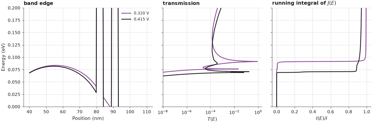
The running integral is close to a single step at both peaks: nearly all the current flows in a narrow energy range around C1, where C1 coincides with an emitter state. The current computed here on the refined grid agrees with the one nemo.thomas_fermi_iv returns.

5. Tracing the critical energies against bias#

The lecture then follows the important energies over the whole bias range: the central resonance C1, the top of the emitter (the maximum of $E_c$ in the emitter spacer), the bottom of the emitter (the band edge in the notch, right at the first barrier), and the notch states E1 and E2.

Code25 lines · cell 18

VT = V[::2]
rows = []
for i in range(0, len(V), 2):
    s = states(i)
    e, g = s["E"]
    c = s["C"]
    rows.append(
        dict(
            top=s["top"],
            bottom=s["bottom"],
            C1=c[0][0] if len(c[0]) else np.nan,
            gC1=c[1][0] if len(c[0]) else np.nan,
            E1=e[0] if s["has_E1"] else np.nan,
            gE1=g[0] if s["has_E1"] else np.nan,
            E2=e[-1] if len(e) > int(s["has_E1"]) else np.nan,
            gE2=g[-1] if len(e) > int(s["has_E1"]) else np.nan,
        )
    )
tr_ = {k: np.array([r[k] for r in rows]) for k in rows[0]}
k32 = int(np.argmin(abs(VT - 0.32)))
print(
    f"from 0 to {VT[k32]:.2f} V: C1 drops {1e3 * (tr_['C1'][0] - tr_['C1'][k32]):.0f} meV, "
    f"emitter top drops {1e3 * (tr_['top'][0] - tr_['top'][k32]):.0f} meV, "
    f"emitter bottom drops {1e3 * (tr_['bottom'][0] - tr_['bottom'][k32]):.0f} meV"
)

from 0 to 0.32 V: C1 drops 108 meV, emitter top drops 31 meV, emitter bottom drops 74 meV

Code17 lines · cell 19

fig, (a1, a2) = plt.subplots(1, 2, figsize=(11, 4))
a1.plot(VT, tr_["C1"], "o", ms=3, color="C3", label="central state C1")
a1.plot(VT, tr_["E1"], "o", ms=3, color=style.OPEN_NEMO, label="emitter state E1")
a1.plot(VT, tr_["E2"], "o", ms=3, color="C2", label="emitter state E2")
a1.plot(VT, tr_["top"], color=style.REFERENCE, label="top of emitter")
a1.plot(VT, tr_["bottom"], color=style.CONTEXT, label="bottom of emitter")
a1.axhline(EF, color=style.OPEN_NEMO, lw=0.8, ls=":", label="$E_F$ (emitter)")
for i in (i_pk, i_2):
    a1.axvline(V[i], color="C3", ls="--", lw=0.8)
a1.set(xlabel="Bias (V)", ylabel="Energy (eV)", ylim=(0, 0.22), title="Critical energies")
a1.legend(fontsize=7)
a2.semilogy(VT, 1e3 * tr_["gC1"], "o", ms=3, color="C3", label="C1")
a2.semilogy(VT, 1e3 * tr_["gE1"], "o", ms=3, color=style.OPEN_NEMO, label="E1")
a2.semilogy(VT, 1e3 * tr_["gE2"], "o", ms=3, color="C2", label="E2")
a2.set(xlabel="Bias (V)", ylabel="Width $\\Gamma$ (meV)", title="Resonance widths")
a2.legend(fontsize=8)
fig.tight_layout();

Slide 16: traces of the central resonance, the emitter band edges and the emitter states against bias — Slide 16. Top: the I–V curve. Bottom: the central state C1 (green), the top (blue) and bottom (orange) of the emitter band edge and the emitter states E1 and E2 against bias. The I–V peaks occur where C1 crosses E2 and E1.

The traces reproduce the lecture's picture:

C1 still falls almost linearly, but by far less than in lecture 11.1: about 0.1 eV for 0.32 V, a lever arm of roughly one third, where the linear-drop model gave one half. Most of the potential is dropped in the depleted collector.
The top of the emitter moves down only a few tens of meV and not linearly: the accumulated emitter charge keeps pushing against being pulled down. The bottom of the emitter, the notch, falls faster, so the triangular well deepens with bias and E1 and later E2 appear in it.
The main current peak (0.32 V) occurs while C1 approaches the top of the emitter, where the broad, loosely bound state E2 sits, and the current collapses between 0.32 and 0.36 V as C1 passes under the top. The second peak (0.415 V) is the crossing of C1 with E1; the two states mix there (anticrossing), which is why their energies and widths jump. Beyond it C1 lies below E1 and only electrons tunnelling through the long emitter hump reach it.
Where E1 is the injector the current is limited: the second peak is four times lower than the main one.

6. Resonance widths: very long-lived emitter states#

The right panel shows the widths. The width of E1 falls exponentially with bias, by more than three orders of magnitude between 0.1 and 0.7 V, because the notch deepens and E1 is enclosed by ever stronger barriers: on the emitter side a hump that is only a few meV higher than E1 but tens of nanometres long, on the other side the AlGaAs barrier. The width of C1 hardly changes, except where it anticrosses E1. The lecture's slide quotes $\Gamma_{C1}=0.4$ meV and $\Gamma_{E1}=8\ \mu$eV at the C1–E1 crossing, and converts the latter into a lifetime of $\tau = \hbar/2\Gamma \approx 40$ ps. The numbers for the present device:

Code16 lines · cell 23

hbar = 6.582119569e-16  # eV s
k2 = int(np.argmin(abs(VT - 0.45)))
for v in (0.3, 0.38, 0.45, 0.5, 0.6):
    k = int(np.argmin(abs(VT - v)))
    print(
        f"{VT[k]:.2f} V: width E1 = {1e6 * tr_['gE1'][k]:8.2f} µeV (hbar/2Gamma = "
        f"{1e12 * hbar / (2 * tr_['gE1'][k]):7.1f} ps),"
        f" width C1 = {1e3 * tr_['gC1'][k]:.2f} meV"
    )
ec, e1 = Ec[2 * k2], tr_["E1"][k2]
hump = emitter & (x > 30) & (ec > e1)
print(
    f"at {VT[k2]:.2f} V the emitter hump around E1 is {np.ptp(x[hump]):.0f} nm long and at most "
    f"{1e3 * (ec[hump].max() - e1):.0f} meV above E1; the first barrier is "
    f"{1e3 * (ec[(x > XB1) & (x < XB1 + 4)].min() - e1):.0f} meV above it"
)

0.30 V: width E1 =   109.73 µeV (hbar/2Gamma =     3.0 ps), width C1 = 0.46 meV
0.38 V: width E1 =    23.81 µeV (hbar/2Gamma =    13.8 ps), width C1 = 0.33 meV
0.45 V: width E1 =    13.63 µeV (hbar/2Gamma =    24.2 ps), width C1 = 0.35 meV
0.50 V: width E1 =     4.33 µeV (hbar/2Gamma =    76.1 ps), width C1 = 0.37 meV
0.60 V: width E1 =     1.43 µeV (hbar/2Gamma =   230.9 ps), width C1 = 0.41 meV
at 0.45 V the emitter hump around E1 is 28 nm long and at most 13 meV above E1; the first barrier is 252 meV above it

E1 narrows from 110 µeV at 0.30 V to 1.4 µeV at 0.60 V, a factor of 77 in 0.3 V. At 0.45 V the hump between E1 and the emitter is 28 nm long and 13 meV higher than E1, and the first AlGaAs barrier is 252 meV above E1: the same shape as the lecture's estimate (about 10 meV over 35 nm on one side, 200 meV over 15 nm on the other). Between 0.45 and 0.5 V the E1 width passes the lecture's 8 µeV, which corresponds to $\hbar/2\Gamma$ of several tens of picoseconds.

Slide 18: bias dependence of the resonance widths of E1, E2 and C1 — Slide 18. Widths (red) and energies (green) against bias. The width of E1 falls exponentially to about 8 µeV ($\tau_{E1} = \hbar/2\Gamma_{E1} = 40$ ps); C1 stays near 0.4 meV. Since $\Gamma_{C1} \gg \Gamma_{E1}$, E1 determines the current at the second peak.

Which width matters for the current? In a picture of two resonances in series, an electron must pass both, and the narrower one limits the flux, like the smaller of two conductances in series. At the second peak $\Gamma_{C1}\gg\Gamma_{E1}$: C1 is a broad bandpass filter looking at a very narrow supply, and E1 determines the current. At the main peak the injecting state E2 is broader than C1 (the slide quotes $\Gamma_{E2}=2$ meV; in the present device it is about 15 meV), so C1 limits the current. "The width of the injector state matters", and with it the shape of the emitter.

The lecturer ends with a question: is it realistic that an electron sits in the emitter notch for tens of picoseconds, in a region with $10^{17}$–$10^{18}$ electrons per cm$^3$ that scatter off each other and off phonons? It is not, and lecture 11.3 adds the missing relaxation.

7. Exploration: the spacer length#

The undoped spacer sets how much potential the emitter and collector absorb and how deep the notch becomes. The cell repeats the Thomas–Fermi I–V for 20, 50 and 100 nm spacers.

Code10 lines · cell 28

fig, ax = plt.subplots(figsize=(6, 3.8))
VS = np.round(np.arange(0.0, 0.9001, 0.01), 3)
for sp, c in zip((20.0, 50.0, 100.0), style.sweep(3)):
    dev = make_rtd(spacer=sp)
    Js = nemo.thomas_fermi_iv(dev, VS, T, charge="all", relaxation=None)["current_density"]
    k = int(np.argmax(np.where(VS < 0.6, Js, 0)))
    print(f"spacer {sp:5.0f} nm: {dev.num_sites} sites, main peak {Js[k]:6.0f} A/cm^2 at {VS[k]:.2f} V")
    ax.plot(VS, Js, color=c, lw=2, label=f"{sp:.0f} nm spacers")
ax.set(xlabel="Bias (V)", ylabel="Current density (A/cm²)", title="Spacer length, Thomas–Fermi, ballistic")
ax.legend();

spacer    20 nm: 452 sites, main peak  11924 A/cm^2 at 0.28 V
spacer    50 nm: 692 sites, main peak   2403 A/cm^2 at 0.32 V
spacer   100 nm: 1092 sites, main peak   1042 A/cm^2 at 0.41 V

Longer spacers move the main peak to higher bias (0.28, 0.32 and 0.41 V for 20, 50 and 100 nm), since more of the applied voltage is dropped across the depleted collector spacer before C1 reaches the emitter states, and they lower the peak current (from about $1.2\times10^4$ to $10^3$ A/cm$^2$), because the emitter electrons have to come over a higher, wider hump. With 20 nm spacers the contacts are so close that the current rises steeply again above 0.5 V, where electrons pass over the low collector barrier region.

Summary#

Real RTDs have heavily doped contacts and undoped spacers to avoid ionized-impurity scattering. Electrons diffusing into the spacers raise the potential: the double barrier floats above the Fermi levels.
The Thomas–Fermi model computes the charge semiclassically from the local band edge and Fermi level and solves it self-consistently with Poisson's equation; it is fast but has no quantum effects.
Under bias the emitter accumulates charge and resists the pull of the collector, the collector depletes, and most of the voltage drops on the collector side. C1 falls by only about a third of the bias.
A triangular notch forms in front of the first barrier. Its quasi-bound states E1 and E2 are probed by C1: each alignment gives an I–V peak, so the I–V has several peaks.
The width of E1 falls exponentially with bias, to microelectronvolts, while C1 keeps about 0.4 meV. The narrower state of a pair limits the current; the lifetimes of tens of picoseconds are unphysical in a heavily doped emitter.

Exercises#

Recompute the I–V at 77 K. Do the notch peaks become sharper or do new ones appear?
Run nemo.thomas_fermi_iv with charge="contacts" (no free charge outside the contacts). How do the band profile at 0.32 V and the I–V change, and why is the notch shallower?
Make the emitter spacer 20 nm and the collector spacer 100 nm (write the layers by hand). Which peak moves, and why?
Fit an exponential to the E1 width between 0.45 and 0.6 V. By how much does each 0.1 V reduce it?