Lecture 23.6

Theory of stress and strain — alloys

In the lecture

A random In$x$Ga${1-x}$As alloy, grown by molecular beam epitaxy (MBE) or MOCVD with the indium fraction set in the growth chamber.
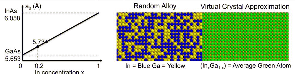
Vegard's law and the virtual crystal approximation: interpolate lattice constant and elastic constants linearly between the binaries, replacing In and Ga by an average 'green' atom.
Is it valid? For the average lattice constant and, roughly, for the elastic constants, yes; locally, no: In–As and Ga–As bonds keep nearly their own lengths (EXAFS), band gaps bow, and at the nanometre scale the disorder of an alloy interface matters.
In${0.2}$Ga${0.8}$As on GaAs has about a fifth of the strain of InAs: layers of 10–20 nm stay pseudomorphic instead of about 1.7 monolayers, enough for a realistic quantum well.

In this notebook

You interpolate the In$x$Ga${1-x}$As parameters with Vegard's law and compare them with open-nemo's Vurgaftman alloy parameters; relax random InGaAs supercells with the Keating valence force field and find that the average lattice follows Vegard's law while the bonds stay bimodal, as EXAFS measures; compute the bowed band gaps of InGaAs and AlGaAs, including the Γ–X crossover of AlGaAs; and tabulate the biaxial strain and stored energy of In$x$Ga${1-x}$As on GaAs as a function of $x$.

Run the notebookEvery number and figure on this page comes from it. Change it, rerun it, take it further.

Download .ipynb View on GitHub

Run it on your own machine

The notebook needs open-nemo (Python ≥ 3.10 and a C++20 compiler; BLAS/LAPACK).

git clone https://github.com/denphi/open-nemo.git && cd open-nemo
python3 -m venv .venv && source .venv/bin/activate
pip install -e ".[notebooks]"
jupyter lab From_Atoms_to_Devices/09_stress_and_strain/23_6_alloys.ipynb

Code9 lines · cell 1

import numpy as np
import matplotlib.pyplot as plt
import opennemo as nemo
from opennemo.visualization import style
from opennemo.models import ema, kp
from opennemo.models import mechanics as M
from opennemo.structures.structure import Structure

style.use(notebook=True)

1. Interpolating between the binaries: Vegard's law#

GaAs and InAs are binaries; mixing them on the group-III sites gives the ternary alloy In$x$Ga${1-x}$As, where $x$ is the fraction of group-III sites occupied by indium. The alloy is grown by molecular beam epitaxy (MBE) or metal-organic chemical vapour deposition (MOCVD), and the ratio of indium to gallium in the growth chamber sets $x$. The atoms are not ordered: which site gets an In and which a Ga is random. The simplest description ignores that and interpolates linearly between the binaries. For the lattice constant this is Vegard's law,

a_0(x) = x\,a_\mathrm{InAs} + (1-x)\,a_\mathrm{GaAs},

and the elastic constants are commonly treated the same way, $C_{ij}(x) = x\,C_{ij}^\mathrm{InAs} + (1-x)\,C_{ij}^\mathrm{GaAs}$. In effect, the blue In and yellow Ga atoms are replaced by one average "green" atom on every group-III site: the virtual crystal approximation (VCA). The result is again a perfect crystal, which all the formulas of Lectures 23.2–23.5 can handle.

Slide 3: Vegard's law and the virtual crystal — Slide 3. Left: the lattice constant of In$_x$Ga$_{1-x}$As interpolated linearly from GaAs (5.653 Å) to InAs (6.058 Å); 5.734 Å at $x = 0.2$. Right: a random alloy of In (blue) and Ga (yellow) atoms, and its virtual crystal of average green atoms.

Code13 lines · cell 3

gaas, inas = kp.material("GaAs"), kp.material("InAs")

def vegard(x, field):
    return x * getattr(inas, field) + (1 - x) * getattr(gaas, field)

x = 0.2
alloy = kp.material("InGaAs", x=x)                                 # Vurgaftman's alloy parameters
print(f"In{x}Ga{1 - x}As      Vegard / VCA      kp.material('InGaAs', x=0.2)")
print(f"a0 (Å)       {10 * vegard(x, 'lattice_constant'):12.4f}   {10 * alloy.lattice_constant:16.4f}")
for f in ("c11", "c12", "c44"):
    print(f"{f.upper()} (GPa)    {vegard(x, f):12.1f}   {getattr(alloy, f):16.1f}")
print(f"C12/C11      {vegard(x, 'c12') / vegard(x, 'c11'):12.3f}   {alloy.c12 / alloy.c11:16.3f}")
print(f"band gap (eV){x * inas.band_gap + (1 - x) * gaas.band_gap:12.3f}   {alloy.band_gap:16.3f}")

In0.2Ga0.8As      Vegard / VCA      kp.material('InGaAs', x=0.2)
a0 (Å)             5.7343             5.7343
C11 (GPa)           114.3              114.3
C12 (GPa)            54.3               54.3
C44 (GPa)            55.9               55.9
C12/C11             0.475              0.475
band gap (eV)       1.209              1.132

For the mechanical parameters the Vurgaftman set, which open-nemo uses for alloys, is itself the linear interpolation: $a_0 = 5.734$ Å, $C_{11} = 114.3$ GPa, $C_{12} = 54.3$ GPa, $C_{12}/C_{11} = 0.475$, the slide's numbers. The band gap is a different matter: linear interpolation gives 1.209 eV at 300 K, the measured alloy has 1.132 eV. Section 2 returns to this.

2. Is this really valid?#

Klimeck answers in three parts. The average lattice constant of InGaAs is close to linear in $x$, and the elastic constants are a reasonable approximation; continuum theory is meant for large objects, and for them Vegard's law works. Locally, it does not: In–As bonds want to be long and Ga–As bonds short, and X-ray absorption experiments (EXAFS) measure two separate bond lengths in the alloy, each close to its binary value, with only the average crystal following the line. And the band gaps are strongly non-linear in $x$ ("bowing"): they must not be interpolated linearly.

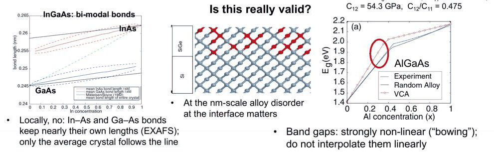
Slide 4: bimodal bonds in InGaAs, disorder in SiGe, and the AlGaAs band gap — Slide 4. Left: measured In–As and Ga–As bond lengths in InGaAs against composition (EXAFS, black) with valence-force-field calculations of Klimeck's group (error bars): the bonds are bimodal. Middle: a 25 % Ge random SiGe alloy, in which atom types and bond lengths fluctuate. Right: the AlGaAs band gap, which a virtual crystal gets wrong, with a kink near 40 % Al.

The bimodal bonds can be reproduced with a valence force field, as on the slide. The cell below builds random In$x$Ga${1-x}$As supercells of 4 × 4 × 4 cubic cells (512 atoms), places In atoms at random on a fraction $x$ of the cation sites, and relaxes all atoms and the supercell size with the Keating force field (Martin's parameters; relax(cell=True) lets the periodic cell "breathe" as NEMO 3-D does). It then measures the relaxed lattice constant and every cation–anion bond.

Code32 lines · cell 5

a_k = {name: M.KEATING_PARAMETERS[name][2] for name in ("GaAs", "InAs")}   # VFF equilibrium (nm)
lat = nemo.structures.lattice.from_material(nemo.structures.materials.load("klimeck2002_sp3d5s")["GaAs"])
unit = lat.conventional_basis / lat.conventional[0, 0]                      # basis in units of a
species0 = list(lat.conventional_species)
N = 4
offsets = np.stack(np.meshgrid(*(np.arange(N),) * 3, indexing="ij"), -1).reshape(-1, 3)

def random_alloy(x, seed=1):
    a_v = x * a_k["InAs"] + (1 - x) * a_k["GaAs"]                             # start from Vegard
    pos = ((offsets[:, None, :] + unit[None]) * a_v).reshape(-1, 3)
    species = species0 * len(offsets)
    cations = [i for i, sp in enumerate(species) if sp == "Ga"]
    for i in np.random.default_rng(seed).choice(cations, int(round(x * len(cations))), replace=False):
        species[i] = "In"
    r = M.relax(M.Keating(Structure(pos, species, np.eye(3) * N * a_v)), tol=1e-6, cell=True)
    box = np.diag(r["periods"])
    X, sp = r["positions"], np.array(species)
    anions = X[sp == "As"]
    bonds = {"Ga": [], "In": []}
    for i in np.flatnonzero(sp != "As"):
        d = anions - X[i]
        d -= box * np.round(d / box)                                            # minimum image
        bonds[sp[i]] += list(np.sort(np.linalg.norm(d, axis=1))[:4])
    return box.mean() / N, a_v, {k: np.array(v) for k, v in bonds.items()}

xs = [0.0, 0.2, 0.4, 0.5, 0.6, 0.8, 1.0]
results = {x: random_alloy(x) for x in xs}
print("  x    a (relaxed)  a (Vegard)    <Ga–As>    <In–As>    VCA bond   (nm)")
for x, (a_rel, a_v, b) in results.items():
    ga = f"{b['Ga'].mean():.5f}" if len(b["Ga"]) else "   –   "
    inn = f"{b['In'].mean():.5f}" if len(b["In"]) else "   –   "
    print(f"{x:4.1f}   {a_rel:.5f}     {a_v:.5f}     {ga:>8s}   {inn:>8s}   {np.sqrt(3) / 4 * a_v:.5f}")

  x    a (relaxed)  a (Vegard)    <Ga–As>    <In–As>    VCA bond   (nm)
 0.0   0.56530     0.56530      0.24478       –      0.24478
 0.2   0.57259     0.57340      0.24559    0.25800   0.24829
 0.4   0.58025     0.58150      0.24639    0.25908   0.25180
 0.5   0.58434     0.58555      0.24670    0.25977   0.25355
 0.6   0.58851     0.58960      0.24703    0.26034   0.25530
 0.8   0.59694     0.59770      0.24789    0.26130   0.25881
 1.0   0.60580     0.60580         –       0.26232   0.26232

Code25 lines · cell 6

fig, (ax1, ax2) = plt.subplots(1, 2, figsize=(10, 4))
xx = np.array(xs)
for el, col, lab in (("In", style.OPEN_NEMO, "In–As"), ("Ga", style.REFERENCE, "Ga–As")):
    m = [results[x][2][el].mean() if len(results[x][2][el]) else np.nan for x in xs]
    s = [results[x][2][el].std() if len(results[x][2][el]) else np.nan for x in xs]
    ax1.errorbar(xx, 10 * np.array(m), yerr=10 * np.array(s), fmt="o-", color=col, capsize=3,
                 label=f"{lab} bonds, Keating random alloy")
ax1.plot(xx, 10 * np.sqrt(3) / 4 * (xx * a_k["InAs"] + (1 - xx) * a_k["GaAs"]), "--", color=style.CONTEXT,
         label="virtual crystal (Vegard)")
ax1.set_xlabel("In fraction x")
ax1.set_ylabel("bond length (Å)")
ax1.set_title("Bonds keep their own lengths")
ax1.set_ylim(2.39, 2.64)
ax1.legend(fontsize=8, loc="lower right")
b = results[0.5][2]
bins = np.linspace(2.42, 2.66, 49)
ax2.hist(10 * b["Ga"], bins=bins, color=style.REFERENCE, alpha=0.8, label="Ga–As")
ax2.hist(10 * b["In"], bins=bins, color=style.OPEN_NEMO, alpha=0.8, label="In–As")
ax2.axvline(10 * np.sqrt(3) / 4 * results[0.5][1], color=style.CONTEXT, ls="--", label="VCA bond")
ax2.set_xlabel("bond length (Å)")
ax2.set_ylabel("number of bonds")
ax2.set_title("In$_{0.5}$Ga$_{0.5}$As: a bimodal distribution")
ax2.legend(fontsize=8)
plt.tight_layout()
plt.show()

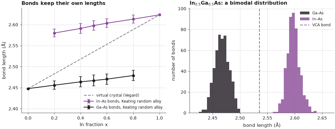
Figure computed by the notebook with open-nemo

The relaxed supercells follow Vegard's law for the lattice constant to within 0.21 %, lying slightly below the line (0.5726 nm at $x = 0.2$ against 0.5734 nm), but their bonds do not follow the virtual crystal at all. At $x = 0.5$ the virtual crystal would have a single bond length of 2.536 Å; the force field gives Ga–As bonds of 2.467 Å and In–As bonds of 2.598 Å, each much closer to its binary value (2.448 and 2.623 Å) than to the average. This is the bimodal distribution EXAFS measures: Ga–As bonds stretch by only 0.019 Å and In–As bonds compress by 0.026 Å, while the bond angles absorb the misfit. The spread within each bond type (the error bars and the histogram) comes from the random neighbourhoods. A virtual crystal is a perfect crystal; a random alloy is not, and in a nanostructure whose wave functions extend over a few nanometres, as in the SiGe example of slide 4, these local fluctuations matter.

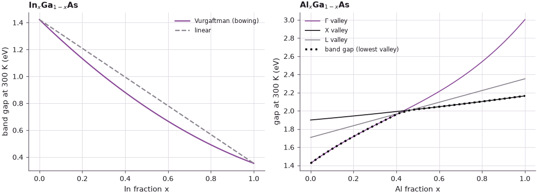
Band gaps are the second failure of linear interpolation. Vurgaftman's parameters, used by kp.material and ema.iii_v_valley_edges, include a bowing term, $E_g(x) = x E_g^\mathrm{B} + (1-x)E_g^\mathrm{A} - b\,x(1-x)$. For AlGaAs a second effect appears: AlAs is an indirect semiconductor whose lowest conduction valley is at X, GaAs a direct one at Γ, and the two valleys cross.

Code26 lines · cell 8

xg = np.linspace(0, 1, 101)
fig, (ax1, ax2) = plt.subplots(1, 2, figsize=(10, 3.8))
eg_ingaas = np.array([kp.material("InGaAs", x=v).band_gap for v in xg])
ax1.plot(xg, eg_ingaas, color=style.OPEN_NEMO, label="Vurgaftman (bowing)")
ax1.plot(xg, xg * inas.band_gap + (1 - xg) * gaas.band_gap, "--", color=style.CONTEXT, label="linear")
ax1.set_xlabel("In fraction x")
ax1.set_ylabel("band gap at 300 K (eV)")
ax1.set_title("In$_x$Ga$_{1-x}$As")
ax1.legend(fontsize=8)
valleys = [ema.iii_v_valley_edges("AlGaAs", v, 300.0) for v in xg]
for key, col in (("Gamma", style.OPEN_NEMO), ("X", style.REFERENCE), ("L", style.CONTEXT)):
    ax2.plot(xg, [vd[key]["gap"] for vd in valleys], color=col, lw=1.2,
             label=f"{key.replace('Gamma', 'Γ')} valley")
eg_algaas = np.array([min(vd[k]["gap"] for k in ("Gamma", "X", "L")) for vd in valleys])
ax2.plot(xg, eg_algaas, "k:", lw=2.5, label="band gap (lowest valley)")
g0, g1 = valleys[0]["Gamma"]["gap"], valleys[-1]["Gamma"]["gap"]
ax2.set_xlabel("Al fraction x")
ax2.set_ylabel("gap at 300 K (eV)")
ax2.set_title("Al$_x$Ga$_{1-x}$As")
ax2.legend(fontsize=8)
plt.tight_layout()
plt.show()
cross = xg[np.argmax([vd["X"]["gap"] < vd["Gamma"]["gap"] for vd in valleys])]
print(f"InGaAs bowing at x = 0.5: linear {0.5 * (inas.band_gap + gaas.band_gap):.3f} eV, "
      f"bowed {kp.material('InGaAs', x=0.5).band_gap:.3f} eV")
print(f"AlGaAs: Γ gap {g0:.3f} → {g1:.3f} eV; the X valley becomes the lowest at x ≈ {cross:.2f}")

InGaAs bowing at x = 0.5: linear 0.888 eV, bowed 0.769 eV
AlGaAs: Γ gap 1.422 → 3.003 eV; the X valley becomes the lowest at x ≈ 0.44

The InGaAs gap bows below the straight line, by 0.119 eV at $x = 0.5$ (0.769 eV against 0.888 eV). In AlGaAs the Γ gap rises from 1.422 eV to 3.003 eV, but the X valley rises much less; it takes over as the lowest conduction valley at $x \approx 0.44$, where the gap has the kink shown on the slide. Beyond it the alloy is an indirect semiconductor. A virtual crystal built from tight-binding parameters by averaging gets these gaps wrong; this course treats random alloys atomistically later.

3. Biaxial strain: InAs against In${0.2}$Ga${0.8}$As on GaAs#

The practical consequence for strain is that $x$ tunes it. With the interpolated parameters, the biaxial-strain formulas of Lecture 23.5 apply unchanged:

Code13 lines · cell 10

def biaxial_table(m):
    e = kp.biaxial_strain(m, gaas.lattice_constant)
    ep, ez = e[0, 0], e[2, 2]
    return [10 * m.lattice_constant, 10 * gaas.lattice_constant, m.c12 / m.c11, 100 * ep, 100 * ez,
            10 * m.lattice_constant * (1 + ez), 100 * (2 * ep + ez), 100 * (ez - ep)]

rows = ["natural a0 of the layer (Å)", "substrate a_s, GaAs (Å)", "C12/C11 of the layer", "ε∥ (%)",
        "ε⊥ (%)", "a⊥ (Å)", "volume: Tr ε (%)", "shape: ε⊥ − ε∥ (%)"]
t_inas, t_alloy = biaxial_table(inas), biaxial_table(alloy)
print(f"{'':30s}{'InAs':>10s}{'In0.2Ga0.8As':>15s}")
for name, v1, v2 in zip(rows, t_inas, t_alloy):
    print(f"{name:30s}{v1:10.3f}{v2:15.3f}")
print(f"ratio of in-plane strains: {t_alloy[3] / t_inas[3]:.3f}")

                                    InAs   In0.2Ga0.8As
natural a0 of the layer (Å)        6.058          5.734
substrate a_s, GaAs (Å)            5.653          5.653
C12/C11 of the layer               0.543          0.475
ε∥ (%)                            -6.686         -1.413
ε⊥ (%)                             7.266          1.343
a⊥ (Å)                             6.499          5.811
volume: Tr ε (%)                  -6.106         -1.483
shape: ε⊥ − ε∥ (%)                13.952          2.755
ratio of in-plane strains: 0.211

These are the slide's numbers: In${0.2}$Ga${0.8}$As on GaAs has $\varepsilon_\parallel = -1.41\,\%$, $\varepsilon_\perp = +1.34\,\%$, $a_\perp = 5.811$ Å, a volume change of −1.48 % and a shape change of +2.76 %, against −6.69 %, +7.27 %, 6.499 Å, −6.11 % and +13.95 % for InAs. With 20 % indium the strain is 0.211 of the InAs strain, about a fifth. Strain is nearly proportional to $x$, since the mismatch is about $x \times 7\,\%$:

Code15 lines · cell 12

xs_s = np.linspace(0, 1, 51)
tabs = np.array([biaxial_table(kp.material("InGaAs", x=v)) if 0 < v < 1 else
                 biaxial_table(gaas if v == 0 else inas) for v in xs_s])
fig, ax = plt.subplots(figsize=(7, 3.8))
for idx, lab, col, ls in ((3, "ε∥", style.OPEN_NEMO, "-"), (4, "ε⊥", style.REFERENCE, "-"),
                          (6, "Tr ε (volume)", style.OPEN_NEMO, "--"),
                          (7, "ε⊥ − ε∥ (shape)", style.REFERENCE, "--")):
    ax.plot(xs_s, tabs[:, idx], color=col, ls=ls, label=lab)
ax.axvline(0.2, color="k", lw=0.8, ls=":")
ax.axhline(0, color="k", lw=0.5)
ax.set_xlabel("In fraction x of the layer")
ax.set_ylabel("strain (%)")
ax.set_title("In$_x$Ga$_{1-x}$As on GaAs (001): x tunes the strain")
ax.legend(fontsize=8, ncol=2)
plt.show()

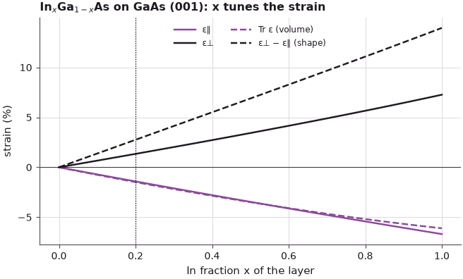
The reduced strain is what makes InGaAs useful. The stored elastic energy grows as the square of the strain (Lecture 23.5), and much thicker layers stay pseudomorphic before islands or misfit dislocations form: about 10–20 nm for In${0.2}$Ga${0.8}$As instead of about 1.7 monolayers for InAs. A strained In${0.2}$Ga${0.8}$As layer between GaAs barriers is therefore a realistic quantum well, the worked example of Lecture 23.7, where the strain finally meets the band edges.

Summary#

Vegard's law and the virtual crystal approximation interpolate the lattice constant and elastic constants linearly: In${0.2}$Ga${0.8}$As has $a_0 = 5.734$ Å, $C_{11} = 114.3$ GPa, $C_{12} = 54.3$ GPa, $C_{12}/C_{11} = 0.475$.
On average this works: relaxed random Keating supercells follow Vegard's lattice constant to 0.21 %.
Locally it fails: the bonds are bimodal (Ga–As 2.467 Å, In–As 2.598 Å at $x = 0.5$ against a single VCA bond of 2.536 Å), as EXAFS measures; and band gaps bow (InGaAs: 0.119 eV at $x = 0.5$; AlGaAs turns indirect at $x \approx 0.44$).
The In fraction tunes the strain: In${0.2}$Ga${0.8}$As on GaAs has $\varepsilon_\parallel = -1.41\,\%$, $\varepsilon_\perp = +1.34\,\%$, about a fifth of InAs, and stays pseudomorphic for 10–20 nm.

Exercises#

Repeat the random-alloy relaxation with three different random seeds at $x = 0.2$. How much do the lattice constant and the mean bond lengths vary from one alloy to the next? How does that change with a larger supercell (N = 6)?
Compute the bond-angle distribution around the As atoms in the $x = 0.5$ supercell. How far do the angles deviate from the ideal 109.47°?
Use kp.biaxial_strain for In$x$Ga${1-x}$As on an InP substrate (kp.material("InP")). At which $x$ is the layer lattice-matched, and when is it under tension?
Plot the AlGaAs valley edges ("edge" instead of "gap") to see which valley the electrons occupy in a GaAs/AlGaAs heterostructure as the Al fraction grows.