

Lecture 24.3
Long-range strain — reducing the electronic domain
In the lecture
- Step 1 repeats the experiment of Lecture 24.2 (electronic structure up to a 20 nm buffer, 9.76 million atoms) and adds the band edges at the centre of the dot from strain calculations alone, which are much cheaper and reach a 24 nm buffer (14.28 million atoms).
- The ground states are not converged, but the band edges at the centre nearly are, and for large buffers the ground states trace them closely.
- Step 2 separates the two domains: freeze the atoms of the largest strain calculation and compute the states in smaller and smaller electronic subdomains, from a 20 nm down to a 4 nm buffer.
- The levels do not change: the wavefunctions reach no deeper than 4 nm into the GaAs and touch fewer than 0.83 million atoms, while the strain acts beyond 24 nm in at least one direction.
- Open questions for Lecture 24.4: which strain direction matters more, vertical or lateral, and what are the right strain boundary conditions?
In this notebook
You redo both steps for the InAs dome of Lecture 24.2 with open-nemo's finite-element strain and the effective-mass model on the local band edges: the ground states and the band edges at the dot's centre for strain domains of up to 40 nm buffer, then the levels in electronic boxes from 16 nm down to 1 nm around the dot with the strain frozen from a 24 nm domain, the decay of the wavefunctions into the GaAs, and the number of atoms each domain needs.
Run it on your own machine
The notebook needs open-nemo (Python ≥ 3.10 and a C++20 compiler; BLAS/LAPACK).
git clone https://github.com/denphi/open-nemo.git && cd open-nemo
python3 -m venv .venv && source .venv/bin/activate
pip install -e ".[notebooks]"
jupyter lab From_Atoms_to_Devices/10_long_range_strain/24_3_reducing_the_electronic_domain.ipynbCode
import time

import numpy as np
import matplotlib.pyplot as plt
import opennemo as nemo
from opennemo.models import kp
from opennemo.solvers import elasticity as el
from opennemo.solvers.poisson import Grid
from opennemo.structures.shapes import Box, Dome
from opennemo.visualization import style

style.use(notebook=True)
T_START = time.time()
1. Step 1: grow the domain and watch the band edges at the centre#
Two calculations of very different cost are involved in a dot simulation. The strain needs only the atom positions, a minimization of a valence force field whose cost grows linearly with the number of atoms. The electronic structure needs the eigenstates of a tight-binding Hamiltonian of 10–20 orbitals per atom, many times more expensive. In 2000 the electronic structure stopped at a 20 nm buffer around the dot (9.76 million atoms), but the strain could go further, and with it the "classical" local band edges at the centre of the dot, which need only the local strain.
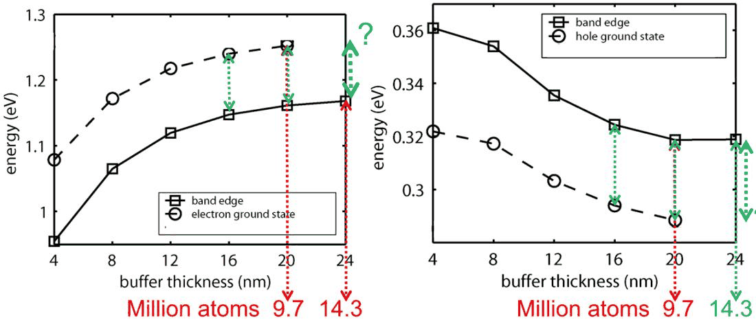 Slide 7: electron and hole ground states (up to 9.7 million atoms) and the band edges at the dot's
centre (up to 14.3 million atoms) against the number of atoms in the domain: the states are not
converged, the centre band edges nearly are, and the states trace them for large buffers. Hypothesis:
for large strain domains the band edge is a good indicator.
The model is that of the previous lectures: finite-element strain with free outer surfaces, 8-band k·p local band edges, single-band effective-mass states (Vurgaftman et al. 2001 parameters, 300 K). As in Lecture 24.2, the hard walls of the electronic box sit \(\min(b, 5\ \mathrm{nm})\) outside the dot; §2 shows that this changes the levels by less than a meV.
Code
GaAs = kp.material("GaAs", temperature=300)            # Vurgaftman et al. (2001), 300 K
InAs = kp.material("InAs", temperature=300)
E0 = GaAs.valence_band_offset                           # energy zero: unstrained GaAs valence-band top


def stiffness(m):
    """Cubic elastic stiffness (GPa, Voigt) of a k·p material."""
    return el.cubic_stiffness(m.c11, m.c12, m.c44)


def misfit(m):
    """Eigenstrain of m on the GaAs reference lattice: a_m / a_GaAs - 1."""
    return m.lattice_constant / GaAs.lattice_constant - 1


for m in (GaAs, InAs):
    print(f"{m.name}: a = {m.lattice_constant:.5f} nm, E_g = {m.band_gap:.3f} eV, "
          f"E_c = {m.valence_band_offset + m.band_gap - E0:+.3f} eV, "
          f"E_v = {m.valence_band_offset - E0:+.3f} eV, "
          f"a_c = {m.ac:+.2f} eV, m_e = {m.electron_mass:.3f} m0")
print(f"InAs misfit on GaAs: {100 * misfit(InAs):.2f} %")
GaAs: a = 0.56532 nm, E_g = 1.422 eV, E_c = +1.422 eV, E_v = +0.000 eV, a_c = -7.17 eV, m_e = 0.067 m0
InAs: a = 0.60583 nm, E_g = 0.354 eV, E_c = +0.564 eV, E_v = +0.210 eV, a_c = -5.08 eV, m_e = 0.026 m0
InAs misfit on GaAs: 7.16 %
Code
VOIGT = [(0, 0), (1, 1), (2, 2), (1, 2), (0, 2), (0, 1)]
_LINEAR = {}


def local_edges(m, eps):
    """Local band edges (eV, from E0) of material m under the strains eps (n, 3, 3): the zone-centre
    eigenvalues of its 8-band k·p Hamiltonian (Bir-Pikus strain terms). Returns E_c, E_HH, E_LH; the
    heavy holes are the valence pair with the least |Z> character (z: growth axis)."""
    if m.name not in _LINEAR:                            # H(eps) = H0 + sum eps_ij D_ij: linear in eps
        h0 = kp.bulk_hamiltonian(m, np.zeros(3), 8)
        d = []
        for i, j in VOIGT:
            u = np.zeros((3, 3))
            u[i, j] = u[j, i] = 1.0
            d.append(kp.bulk_hamiltonian(m, np.zeros(3), 8, strain=u) - h0)
        _LINEAR[m.name] = h0, np.array(d)
    h0, d = _LINEAR[m.name]
    v = np.stack([eps[:, i, j] for i, j in VOIGT], -1)
    w, u = np.linalg.eigh(h0[None] + np.einsum("na,aij->nij", v, d))
    z = np.abs(u[:, 3, 2:6]) ** 2 + np.abs(u[:, 7, 2:6]) ** 2   # basis S, X, Y, Z per spin
    order = np.argsort(z, axis=1)
    top = w[:, 2:6]
    e_hh = np.take_along_axis(top, order[:, :2], 1).max(1)
    e_lh = np.take_along_axis(top, order[:, 2:], 1).max(1)
    return w[:, 6] - E0, e_hh - E0, e_lh - E0


def region_at(result, points):
    """Region index (0: the GaAs matrix, >0: the dot) of the finite-element cell containing each
    point: the cell whose material local_strain_at measures the strain against."""
    p = result.problem
    ids = []
    for d, a in enumerate(p.grid.axes):
        x = points[:, d]
        if p.periodic[d]:
            x = a[0] + np.mod(x - a[0], a[-1] - a[0])
        ids.append(np.clip(np.searchsorted(a, x, side="right") - 1, 0, len(a) - 2))
    return p.material[np.ravel_multi_index(tuple(ids), p.cell_shape)]


eps_test = np.array([[-0.05, 0.01, 0.0], [0.01, -0.05, 0.0], [0.0, 0.0, 0.04]])
direct = np.linalg.eigvalsh(kp.bulk_hamiltonian(InAs, np.zeros(3), 8, strain=eps_test)) - E0
print("direct 8-band:  E_c, top valence =", np.round(direct[[6, 5]], 5))
print("local_edges:    E_c, E_HH, E_LH  =", np.round(np.ravel(local_edges(InAs, eps_test[None])), 5))
direct 8-band:  E_c, top valence = [0.86859 0.32936]
local_edges:    E_c, E_HH, E_LH  = [0.86859 0.32936 0.1134 ]
Code
HB2M = 0.0380998                                         # hbar^2 / 2 m0 (eV nm^2)


def bdd_hamiltonian(shape, h, inv_mass, potential):
    """Single-band BenDaniel-Duke operator -div (hbar^2 / 2m) grad + V on a box grid of spacings h
    (nm) with hard walls; inv_mass (n, 3): m0/m along x, y, z at each point."""
    import scipy.sparse as sp
    n = int(np.prod(shape))
    idx = np.arange(n).reshape(shape)
    diag = np.asarray(potential, dtype=float).copy()
    rows, cols, vals = [], [], []
    for ax in range(3):
        a = np.take(idx, range(shape[ax] - 1), axis=ax).ravel()
        b = np.take(idx, range(1, shape[ax]), axis=ax).ravel()
        t = HB2M * 0.5 * (inv_mass[a, ax] + inv_mass[b, ax]) / h[ax] ** 2
        rows += [a, b]
        cols += [b, a]
        vals += [-t, -t]
        np.add.at(diag, a, t)
        np.add.at(diag, b, t)
        for wall in (np.take(idx, [0], axis=ax).ravel(), np.take(idx, [shape[ax] - 1], axis=ax).ravel()):
            diag[wall] += HB2M * inv_mass[wall, ax] / h[ax] ** 2   # psi = 0 one step outside
    off = sp.coo_matrix((np.concatenate(vals), (np.concatenate(rows), np.concatenate(cols))), shape=(n, n))
    return off.tocsr() + sp.diags(diag)


def hole_inv_mass(m):
    """Heavy-hole m0/m in the plane (gamma1 + gamma2) and along z (gamma1 - 2 gamma2)."""
    return np.array([m.gamma1 + m.gamma2, m.gamma1 + m.gamma2, m.gamma1 - 2 * m.gamma2])


def dot_levels(result, dot, lo, hi, h=(1.0, 1.0, 0.5), num=1, holes=True):
    """Lowest electron and highest hole levels (eV, from E0) of a dot of material `dot` in GaAs, in
    the hard-wall box lo..hi (nm) on a grid of spacings h, with the strain and the regions of the
    finite-element `result`. Returns a dict with the levels, the grid and the band edges on it."""
    axes = [np.arange(lo[i] + h[i] / 2, hi[i], h[i]) for i in range(3)]
    shape = tuple(len(a) for a in axes)
    pts = np.stack(np.meshgrid(*axes, indexing="ij"), -1).reshape(-1, 3)
    ind = region_at(result, pts) > 0
    eps = result.local_strain_at(pts)
    ec, ev = np.empty(len(pts)), np.empty(len(pts))
    for m, sel in ((GaAs, ~ind), (dot, ind)):
        c, hh, lh = local_edges(m, eps[sel])
        ec[sel], ev[sel] = c, np.maximum(hh, lh)
    inv_me = 1.0 / np.where(ind, dot.electron_mass, GaAs.electron_mass)
    re = nemo.eigenstates(bdd_hamiltonian(shape, h, np.repeat(inv_me[:, None], 3, 1), ec), num=num)
    out = {"e": np.sort(re["energies"]), "e_states": re, "points": pts, "shape": shape, "axes": axes,
           "ec": ec, "ev": ev, "inside": ind}
    if holes:                                            # holes: lowest states of (kinetic - E_v)
        inv_mh = np.where(ind[:, None], hole_inv_mass(dot)[None], hole_inv_mass(GaAs)[None])
        rh = nemo.eigenstates(bdd_hamiltonian(shape, h, inv_mh, -ev), num=num)
        out["h"], out["h_states"] = -np.sort(rh["energies"]), rh
    return out


def graded_axis(lo, hi, core_lo, core_hi, h, h_max=2.0, growth=1.25):
    """Grid nodes from lo to hi (nm): spacing h on [core_lo, core_hi] around the dot, growing by
    `growth` per cell outside it up to h_max. Elasticity has no length scale, so the far buffer
    needs no fine grid."""
    def grow(start, end, sign):
        pts, x, s = [], start, h
        while True:
            s = min(s * growth, h_max)
            x += sign * s
            if (x >= end - 0.3 * s) if sign > 0 else (x <= end + 0.3 * s):
                return pts + [end]
            pts.append(x)
    core = list(np.arange(core_lo, core_hi + 1e-9, h))
    return np.array(grow(core_lo, lo, -1)[::-1] + core + grow(core_hi, hi, +1))
Code
R, H = 15.0, 5.0
dome = Dome((0, 0, 0), (R, R, H))                                   # InAs, base at z = 0
CENTRE = np.array([[0.0, 0.0, H / 2]])


def strain_free(b):
    """The InAs dome in a GaAs box with buffer b (nm) on all six sides, free outer surfaces."""
    xa = graded_axis(-R - b, R + b, -R - 1, R + 1, 1.0)
    za = graded_axis(-b, H + b, -1, H + 1, 0.5)
    return el.Elasticity.from_regions(Grid(xa, xa, za), [(None, stiffness(GaAs), 0.0),
                                                         (dome, stiffness(InAs), misfit(InAs))]).solve()


def box(e):
    """Electronic box reaching e (nm) beyond the dot's bounding box in every direction."""
    return (-R - e, -R - e, -e), (R + e, R + e, H + e)


def atoms(e):
    return 8 * (2 * R + 2 * e) ** 2 * (H + 2 * e) / 0.56532**3


t0 = time.time()
strain, centre = {}, {}
for b in range(4, 41, 4):                                           # strain only: cheap
    strain[b] = strain_free(b)
    ec, hh, lh = local_edges(InAs, strain[b].local_strain_at(CENTRE))
    centre[b] = (ec[0], max(hh[0], lh[0]))
t_strain = time.time() - t0
t0 = time.time()
step1 = {b: dot_levels(strain[b], InAs, *box(min(b, 5.0))) for b in (4, 8, 12, 16, 20)}
t_step1 = time.time() - t0
print(" b (nm)   atoms (M)    e1      E_c(centre)   e1 - E_c     h1      E_v(centre)   E_v - h1")
for b in strain:
    line = f"{b:6d}   {atoms(b) / 1e6:8.2f}  "
    if b in step1:
        e1, h1 = step1[b]["e"][0], step1[b]["h"][0]
        line += (f"  {e1:.4f}    {centre[b][0]:.4f}      {e1 - centre[b][0]:.4f}     {h1:.4f}    "
                 f"{centre[b][1]:.4f}      {centre[b][1] - h1:.4f}")
    else:
        line += f"     --      {centre[b][0]:.4f}         --          --     {centre[b][1]:.4f}"
    print(line)
print(f"{len(strain)} strain fields in {t_strain:.1f} s; "
      f"electronic structure for 5 buffers in {t_step1:.1f} s")
 b (nm)   atoms (M)    e1      E_c(centre)   e1 - E_c     h1      E_v(centre)   E_v - h1
     4       0.83    1.0460    0.8330      0.2129     0.2964    0.3692      0.0728
     8       1.97    1.1156    0.9130      0.2026     0.2861    0.3520      0.0659
    12       3.74    1.1471    0.9494      0.1977     0.2731    0.3316      0.0584
    16       6.30    1.1619    0.9658      0.1961     0.2654    0.3207      0.0554
    20       9.76    1.1695    0.9740      0.1955     0.2610    0.3151      0.0541
    24      14.28       --      0.9785         --          --     0.3120
    28      19.98       --      0.9811         --          --     0.3101
    32      27.00       --      0.9827         --          --     0.3089
    36      35.47       --      0.9838         --          --     0.3082
    40      45.54       --      0.9845         --          --     0.3076
10 strain fields in 10.3 s; electronic structure for 5 buffers in 6.5 s
Code
bs, b1 = np.array(list(strain)), np.array(list(step1))
fig, axes = plt.subplots(1, 2, figsize=(11, 3.8))
for ax, k, lab, cl in ((axes[0], "e", "electron", "$E_c$"), (axes[1], "h", "hole", "$E_v$")):
    j = 0 if k == "e" else 1
    ax.plot(atoms(b1) / 1e6, [step1[b][k][0] for b in b1],
            **style.series(points=True, label=f"{lab} ground state"))
    ax.plot(atoms(bs) / 1e6, [centre[b][j] for b in bs], marker=".", **style.series(variant=1,
            label=f"{cl} at the dot's centre (strain only)"))
    ax.axvline(atoms(20) / 1e6, **style.series("context", ls=":"))
    ax.set(xscale="log", xlabel="atoms in the strain domain (millions)", ylabel=f"{lab} energy (eV)",
           title=f"{lab}s: buffer 4 to 40 nm")
    ax.legend(frameon=False, fontsize=8)
fig.tight_layout()
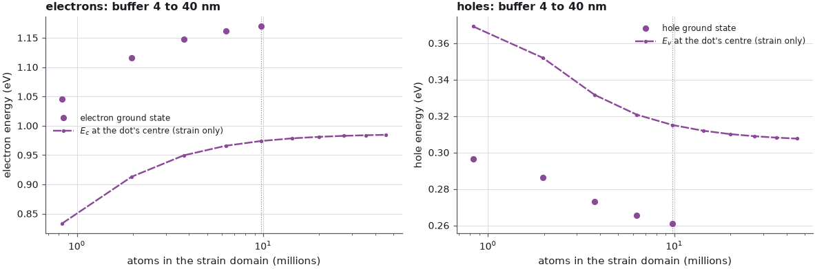
Up to the 20 nm buffer (dotted line, 9.76 million atoms) the picture is the lecture's. The ground states move a lot, by 124 meV (electron) and 35 meV (hole), but they do so together with the band edges at the centre of the dot: \(e_1 - E_c(\text{centre})\) settles at 0.196 eV and \(E_v(\text{centre}) - h_1\) at 0.055 eV for the larger buffers. The confinement energy is set by the dot; the strain domain shifts the whole well.
The strain-only curve, which is cheap, shows how much farther the strain reaches. Between the 20 nm and the 40 nm buffer the conduction band edge at the centre still rises by about 10 meV, more slowly with every step but without a plateau, and the domain has grown to 46 million atoms. With free outer surfaces the dot keeps pushing the ever larger block apart (Lecture 24.2); with the hypothesis that the ground state follows the band edge, the remaining error of the 20 nm calculation can be estimated from strain calculations alone.
2. Step 2: freeze the strain, shrink the electronic domain#
The second step answers the other question: how far does the electronic wavefunction reach? Start from the strain of the largest domain, freeze the atoms there, and compute the states in subdomains around the dot that get smaller and smaller. As long as the wavefunction fits inside the subdomain, its energy cannot change.
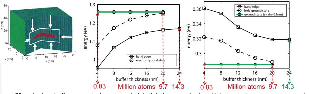 Slide 13: with the atoms frozen from the 24 nm strain calculation (14.3 million atoms), the electron and
hole ground states (stars) stay constant as the electronic domain shrinks from a 20 nm to a 4 nm buffer
(0.83 million atoms). At 20 nm the new hole state lies below that of step 1: the strain of the larger
domain is more relaxed.
Here the strain is that of the 24 nm free-surface calculation of §1, and the electronic box shrinks from 16 nm (284,000 grid points; a 20 nm box would cost as much as all the others together) to 1 nm.
Code
frozen = strain[24]
t0 = time.time()
step2 = {e: dot_levels(frozen, InAs, *box(e)) for e in (16, 12, 8, 6, 4, 3, 2, 1)}
t_step2 = time.time() - t0
ref = step2[16]
print(" box (nm)  grid points   atoms (M)     e1       h1     e1 - e1(16)  h1 - h1(16)")
for e, lv in step2.items():
    print(f"{e:8d}  {np.prod(lv['shape']):10,d}   {atoms(e) / 1e6:8.2f}   {lv['e'][0]:.4f}   {lv['h'][0]:.4f}"
          f"   {1e3 * (lv['e'][0] - ref['e'][0]):+7.2f} meV  {1e3 * (lv['h'][0] - ref['h'][0]):+7.2f} meV")
print(f"step 1 at b = 20 nm: e1 = {step1[20]['e'][0]:.4f} eV, h1 = {step1[20]['h'][0]:.4f} eV "
      f"({t_step2:.1f} s)")

es = np.array(list(step2))
fig, axes = plt.subplots(1, 2, figsize=(11, 3.6))
for ax, k, lab in ((axes[0], "e", "electron"), (axes[1], "h", "hole")):
    ax.plot(es, [step2[e][k][0] for e in es], marker="*", ms=9,
            **style.series(label="step 2: strain of the 24 nm domain, frozen"))
    ax.plot(b1, [step1[b][k][0] for b in b1], marker="o", **style.series(variant=1,
            label="step 1: strain and electrons, same buffer"))
    ax.set(xlabel="buffer of the electronic domain (nm)", ylabel=f"{lab} ground state (eV)", title=f"{lab}s")
    ax.legend(frameon=False, fontsize=8)
fig.tight_layout()
 box (nm)  grid points   atoms (M)     e1       h1     e1 - e1(16)  h1 - h1(16)
      16     284,456       6.30   1.1737   0.2584     +0.00 meV    +0.00 meV
      12     169,128       3.74   1.1737   0.2584     +0.00 meV    -0.00 meV
       8      88,872       1.97   1.1737   0.2584     +0.00 meV    -0.00 meV
       6      59,976       1.33   1.1737   0.2584     +0.02 meV    -0.00 meV
       4      37,544       0.83   1.1740   0.2584     +0.35 meV    -0.00 meV
       3      28,512       0.63   1.1751   0.2584     +1.47 meV    -0.01 meV
       2      20,808       0.46   1.1801   0.2583     +6.47 meV    -0.10 meV
       1      14,336       0.32   1.2053   0.2574    +31.68 meV    -1.02 meV
step 1 at b = 20 nm: e1 = 1.1695 eV, h1 = 0.2610 eV (22.5 s)
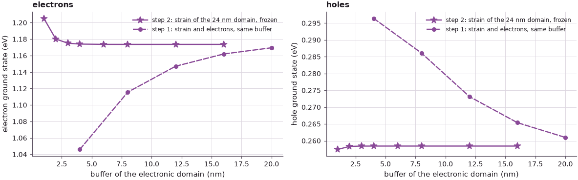
With the strain frozen, the electron and hole levels are the same to within 0.4 meV for every electronic box from 16 nm down to 4 nm; only at 2 nm does the electron rise by 6 meV, and at 1 nm by 32 meV, when the hard walls start to squeeze its wavefunction. The two curves of the figure tell apart what the domain size does to the two physical problems: shrinking the strain domain (step 1) moves the levels by more than 100 meV, shrinking the electronic domain (step 2) does nothing until it cuts into the wavefunction. As on the slide, the frozen-strain hole lies below the step-1 hole at 20 nm (here by 3 meV): the 24 nm domain is more relaxed.
3. How far does the wavefunction reach?#
The 8 nm box holds the ground states with room to spare. The fraction of \(|\psi|^2\) that lies more than a distance \(d\) outside the dot's bounding box, and cuts through the two densities, show how far they reach into the GaAs.
Code
lv = step2[8]
p = lv["points"]
outside = np.max(np.stack([np.abs(p[:, 0]) - R, np.abs(p[:, 1]) - R, -p[:, 2], p[:, 2] - H]), axis=0)
d = np.linspace(0, 6, 61)
fig, axes = plt.subplots(1, 3, figsize=(13, 3.6), gridspec_kw={"width_ratios": [1, 1.2, 1.2]})
for k, (key, lab) in enumerate((("e_states", "electron"), ("h_states", "hole"))):
    rho = np.abs(lv[key]["vectors"][:, 0]) ** 2
    rho /= rho.sum()
    beyond = np.array([rho[outside > x].sum() for x in d])
    axes[0].semilogy(d, beyond, **style.series(variant=k, label=lab))
    print(f"{lab:8s}: weight inside the dot's bounding box {rho[outside <= 0].sum():.3f}; beyond 2 nm "
          f"{np.interp(2, d, beyond):.1e}, beyond 4 nm {np.interp(4, d, beyond):.1e}")
    grid = rho.reshape(lv["shape"])[:, lv["shape"][1] // 2, :]           # the x-z plane through the axis
    x_ax, z_ax = lv["axes"][0], lv["axes"][2]
    im = axes[1 + k].pcolormesh(x_ax, z_ax, grid.T / grid.max(), cmap=style.MAGNITUDE, shading="nearest")
    xs = np.linspace(-R, R, 200)
    axes[1 + k].plot(xs, H * np.sqrt(np.clip(1 - (xs / R) ** 2, 0, 1)), **style.series("context", lw=1.2))
    axes[1 + k].plot([-R, R], [0, 0], **style.series("context", lw=1.2))
    axes[1 + k].set(xlabel="x (nm)", ylabel="z (nm)", title=f"{lab} density, y = 0 (8 nm box)", aspect=2)
    fig.colorbar(im, ax=axes[1 + k], shrink=0.8, label="|ψ|² / max")
axes[0].set(xlabel="distance d outside the dot's bounding box (nm)", ylabel="weight of |ψ|² beyond d",
            title="how far the states reach", ylim=(1e-9, 1))
axes[0].legend(frameon=False)
fig.tight_layout()
print(f"electronic domain with a 4 nm buffer: {atoms(4) / 1e6:.2f} million atoms; "
      f"strain domain with a 24 nm buffer: {atoms(24) / 1e6:.2f} million")
print(f"notebook run time: {time.time() - T_START:.0f} s")
electron: weight inside the dot's bounding box 0.868; beyond 2 nm 7.1e-03, beyond 4 nm 4.1e-04
hole    : weight inside the dot's bounding box 0.972; beyond 2 nm 2.0e-04, beyond 4 nm 3.1e-06
electronic domain with a 4 nm buffer: 0.83 million atoms; strain domain with a 24 nm buffer: 14.28 million
notebook run time: 40 s
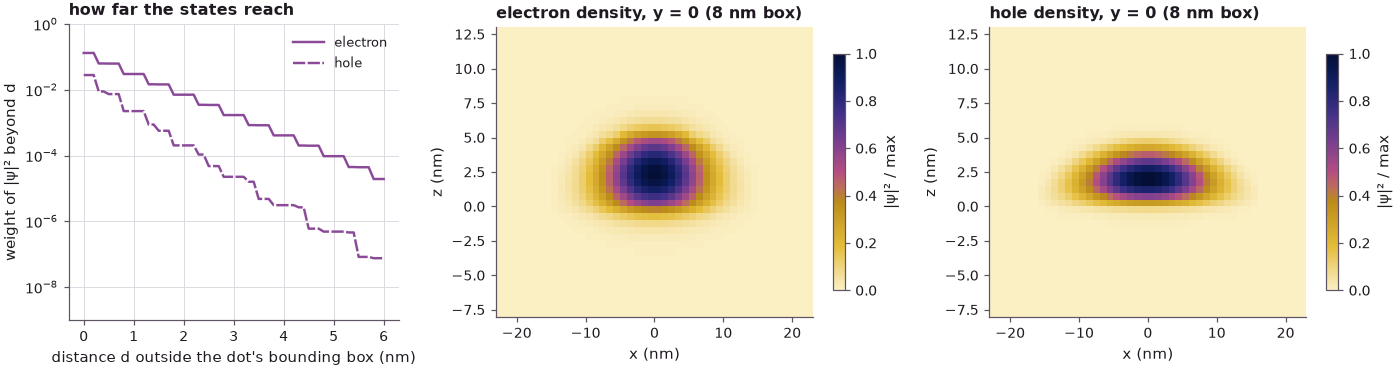
Both states sit inside the dot: the electron (87 % of it inside the dot's bounding box) fills its centre, the heavier hole (97 %) is flatter. Their tails decay exponentially into the GaAs, by about a factor of ten per 1.6 nm for the electron and per 1.1 nm for the hole: 4 × 10⁻⁴ of the electron and 3 × 10⁻⁶ of the hole lie more than 4 nm outside the dot, too little to move the energy by more than 0.4 meV (step 2). That is the lecture's answer: the wavefunction does not go deeper than about 4 nm into the GaAs, and an electronic domain of 0.83 million atoms holds it. The strain, by contrast, still changes the band edges beyond a 24 nm buffer, a domain of 14.3 million atoms. The numbers come from a continuum model, so the absolute decay lengths depend on the effective masses, but the separation of scales does not.
The practical consequence is the recipe of NEMO 3-D: compute the strain in a large domain, where atoms are cheap, and the electronic structure in a small one around the dot. Two questions remain for Lecture 24.4: does the strain matter more along the growth direction or in the plane, and what boundary conditions should replace the free outer surfaces?
Summary#
- Strain domains are much cheaper than electronic domains: the strain and the band edges at the dot's centre can be computed for buffers far beyond what the electronic structure can afford.
- As the domain grows, the ground states are not converged, but they follow the band edges at the dot's centre: \(e_1 - E_c\) and \(E_v - h_1\) settle for buffers above about 12 nm.
- With the strain frozen from a 24 nm domain, the levels do not change as the electronic box shrinks from 16 nm to 4 nm: the wavefunction reaches no more than about 4 nm into the GaAs, a domain of 0.83 million atoms.
- The strain reaches beyond a 24 nm buffer (14.3 million atoms): electronic and strain domains should be chosen separately.
Exercises#
- Repeat step 2 for the In${0.6}$Ga${0.4}$As dome (
kp.material("InGaAs", x=0.6, temperature=300)). Does the alloy's lighter confinement let the electron reach further into the GaAs? - Freeze the strain of the 8 nm domain instead of the 24 nm one and shrink the electronic box. Which conclusion of step 2 still holds, and which number changes?
- Compute the first excited electron state (
num=2indot_levels) and its decay into the GaAs. How small can the electronic box be for it?
Further reading#
- Lecture 24.2: expanding the strain domain, 24.4: boundary conditions and dot configurations
- Lecture 23.7: from strain to band edges
- NEMO 3-D in 2002 (strain and electronic domains of a dome dot)
- Self-assembled InAs/GaAs quantum dots: strain and confinement
- G. Klimeck, F. Oyafuso, T. B. Boykin, R. C. Bowen and P. von Allmen, "Development of a nanoelectronic 3-D (NEMO 3-D) simulator for multimillion atom simulations and its application to alloyed quantum dots", CMES 3, 601 (2002).
- G. Klimeck, S. S. Ahmed, H. Bae, N. Kharche, S. Clark, B. Haley, S. Lee, M. Naumov, H. Ryu, F. Saied, M. Prada, M. Korkusinski, T. B. Boykin and R. Rahman, "Atomistic simulation of realistically sized nanodevices using NEMO 3-D — Part I: Models and benchmarks", IEEE Trans. Electron Devices 54, 2079 (2007).