

Lecture 1.2
Basic device operation — raising 1,000 questions
In the lecture
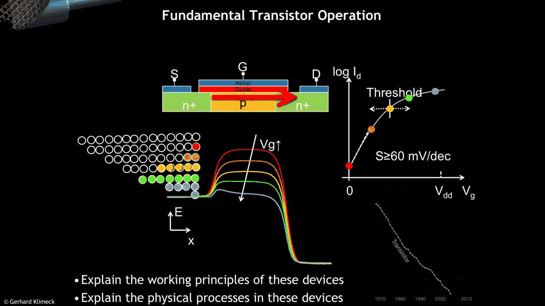
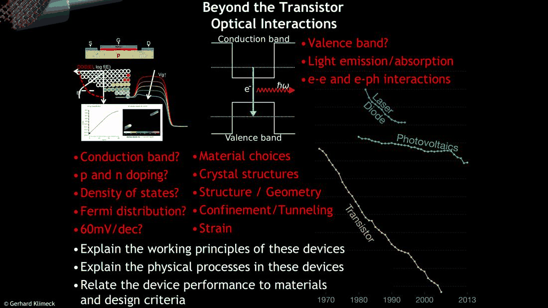
- the textbook picture of a MOSFET: n⁺ source and drain, a p channel, an oxide and a metal gate
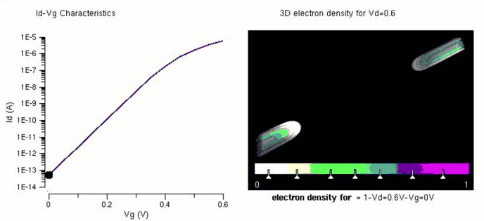
- the conduction band along the channel, a barrier that the gate voltage raises and lowers
- \(\log I_d\) against \(V_g\): the threshold, and a subthreshold swing \(S \geq 60\) mV/dec
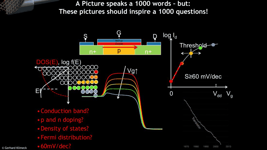
- "a picture speaks 1000 words — these pictures should inspire 1000 questions": conduction band, doping, density of states, Fermi distribution, 60 mV/dec; materials, crystal structure, geometry, confinement and tunneling, strain; valence band, light, electron–electron and electron–phonon interactions
- the learning outcomes: explain the working principles and physical processes of these devices, and relate their performance to materials and design
In this notebook
we turn the slide pictures into calculations. A one-dimensional
effective-mass model of the channel (a barrier whose height the gate sets, ballistic transmission
from open-nemo's Transport, the Landauer current) reproduces the band diagram and the
\(\log I_d\)–\(V_g\) curve, shows where the 60 mV/dec comes from and when it breaks, and shows that
tunneling through a short barrier spoils it. A self-consistent 2 nm silicon gate-all-around
nanowire transistor then gives the same curve for a three-dimensional device, and a GaAs quantum
well gives the photon energy of the optical transition on the last slide.
Run it on your own machine
The notebook needs open-nemo (Python ≥ 3.10 and a C++20 compiler; BLAS/LAPACK).
git clone https://github.com/denphi/open-nemo.git && cd open-nemo
python3 -m venv .venv && source .venv/bin/activate
pip install -e ".[notebooks]"
jupyter lab From_Atoms_to_Devices/01_introduction/01_2_basic_device_operation.ipynbCode
import numpy as np
import matplotlib.pyplot as plt
import opennemo as nemo
from opennemo.visualization import style

style.use(notebook=True)
from scipy.linalg import eigh_tridiagonal
from opennemo.structures.materials import EffectiveMassMaterial, effective_mass

KB = nemo.core.units.KB            # Boltzmann constant (eV/K)
H2M0 = nemo.core.units.HBAR2_2M0   # ħ²/2m₀ (eV nm²)
1. The transistor as a gate-controlled barrier#
The slide draws a planar MOSFET: two heavily doped n⁺ regions (source S and drain D) on either side of a p-type channel, covered by a thin oxide and a metal gate. Electrons enter from the source, cross the channel and leave through the drain. Along the channel the conduction band forms a barrier: the n⁺ source and drain have their band edge near the Fermi level, the p region pushes it up. A positive gate voltage \(V_g\) pulls the barrier down (the colored curves, from red to blue), a drain voltage lowers the drain side. The electrons in the source (the colored circles) that are above the barrier top pass; the others are reflected.
The simplest model that keeps this physics is one-dimensional. The channel is a stretch of silicon, described by an effective mass \(m^* = 0.19\,m_0\) (the transverse mass of the Δ valleys whose light direction lies along the channel). Its band edge \(E_c(x)\) is given by hand: 10 nm of source at \(E_c = 0\), a channel of length \(L_g\) whose top sits at \(E_{top} = E_{top,0} - \alpha V_g\), and 10 nm of drain at \(E_c = -V_d\), joined by smooth steps 1 nm wide. \(\alpha \leq 1\) is the gate coupling, the fraction of the gate voltage that reaches the channel. The source Fermi level is \(\mu_S = 50\) meV above its band edge and the drain's is \(\mu_D = \mu_S - qV_d\). Electrons cross ballistically, with the transmission \(T(E)\) that open-nemo computes for this potential, and the current of the single transverse mode is the Landauer integral
No electrostatics is solved here: the barrier is imposed. Section 4 adds it.
Code
si = EffectiveMassMaterial("Si, Δ valley (m_t along the channel)", mass=0.19, eps_r=11.9)
LSD, DX, MU, VD, TOP0 = 10.0, 0.2, 0.05, 0.3, 0.4   # nm, nm, eV, V, eV


def step(z):
    return 0.5 * (1.0 + np.tanh(z))


def band_edge(x, lg, top, vd, w=1.0):
    # E_c(x): source at 0, a channel barrier of height `top` and length lg, drain at -vd (eV)
    x1, x2 = LSD, LSD + lg
    return top * (step((x - x1) / w) - step((x - x2) / w)) - vd * step((x - x2) / w)


def channel(lg):
    return nemo.Heterostructure1D([nemo.Layer(si, 2 * LSD + lg)], spacing=DX)


def id_vg(lg, vg, alpha=1.0, vd=VD, temp=300.0):
    # ballistic drain current (A) of one transverse mode at each gate voltage
    dev = channel(lg)
    tr, kt, current = nemo.Transport(dev.hamiltonian), KB * temp, []
    for v in vg:
        top = TOP0 - alpha * v
        u = band_edge(dev.x, lg, top, vd)
        e = np.linspace(-vd + 1e-3, max(top, MU) + 25 * kt, 800)
        current.append(nemo.landauer_current(e, tr.transmission(e, potential=u), MU, MU - vd, temp))
    return np.array(current)


def swing(vg, current, n=6):
    # subthreshold swing (mV/dec) from a straight-line fit of V_g against log10 I over the first n points
    return 1e3 * np.polyfit(np.log10(current[:n]), vg[:n], 1)[0]


vg = np.linspace(0.0, 0.5, 26)
i30 = id_vg(30.0, vg)

dev = channel(30.0)
fig, (ax1, ax2) = plt.subplots(1, 2, figsize=(11, 4))
cols = style.sweep(6)
for c, v in zip(cols, np.arange(0.0, 0.51, 0.1)):
    ax1.plot(dev.x, band_edge(dev.x, 30.0, TOP0 - v, VD), color=c, label=f"$V_g$ = {v:.1f} V")
ax1.axhline(MU, color=style.CONTEXT, ls="--", lw=1)
ax1.text(1, MU + 0.015, r"$\mu_S$", fontsize=9)
ax1.set(xlabel="position along the channel x (nm)", ylabel="conduction band edge $E_c$ (eV)")
ax1.legend(fontsize=8)
ax2.semilogy(vg, i30, color=style.OPEN_NEMO, label="open-nemo, $L_g$ = 30 nm")
ax2.semilogy(vg, i30[0] * 10 ** (vg / (KB * 300 * np.log(10))), color=style.REFERENCE, ls="--",
             lw=1, label="60 mV/dec (kT ln10 / q)")
ax2.set(xlabel="gate voltage $V_g$ (V)", ylabel="drain current $I_d$ (A)", ylim=(1e-13, 1e-5))
ax2.legend(fontsize=8)
fig.tight_layout()
print(f"I_d at V_g = 0: {i30[0]:.2e} A;  at 0.5 V: {i30[-1]:.2e} A;  ratio {i30[-1] / i30[0]:.1e}")
print(f"subthreshold swing: {swing(vg, i30):.1f} mV/dec;  kT ln(10)/q at 300 K = "
      f"{1e3 * KB * 300 * np.log(10):.1f} mV/dec")
ceiling = nemo.core.units.G0 * KB * 300 * np.log1p(np.exp(MU / (KB * 300)))   # (2q/h) kT ln(1 + e^(mu/kT))
print(f"one-mode ceiling (2q/h) kT ln(1 + exp(mu_S/kT)) = {ceiling:.2e} A")
I_d at V_g = 0: 1.79e-12 A;  at 0.5 V: 3.72e-06 A;  ratio 2.1e+06
subthreshold swing: 59.3 mV/dec;  kT ln(10)/q at 300 K = 59.5 mV/dec
one-mode ceiling (2q/h) kT ln(1 + exp(mu_S/kT)) = 4.14e-06 A
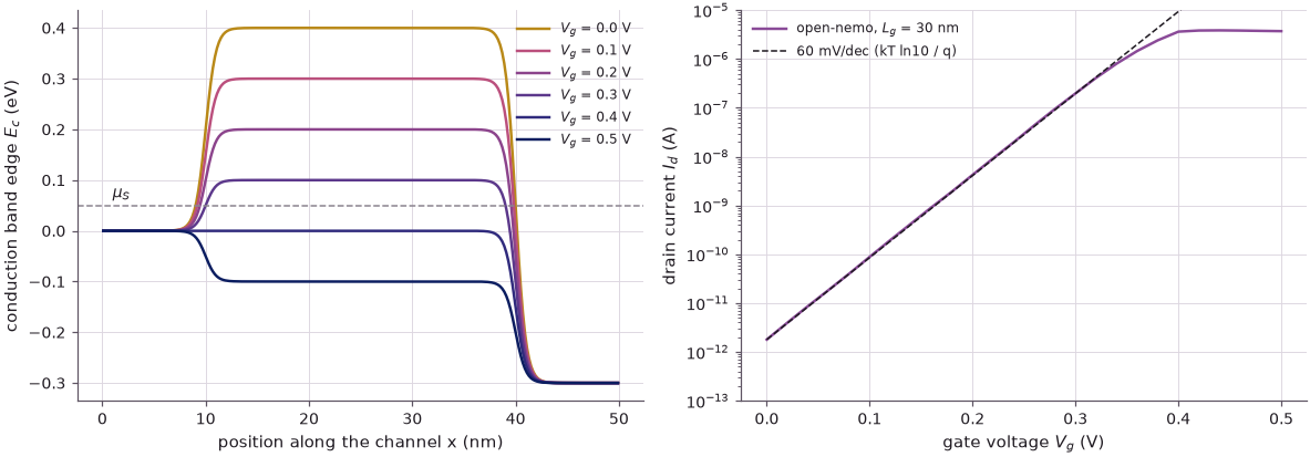
The left panel is the band diagram of the slide, computed. On the right the current rises in a straight line on the log scale, by six orders of magnitude between \(V_g = 0\) and 0.4 V, then saturates once the barrier top drops below the source Fermi level: the threshold. The slope below threshold is 59.3 mV per decade; the dashed line is \(k_BT\ln 10/q = 59.5\) mV/dec. Above threshold the current, 3.7 µA at 0.5 V, approaches the ceiling of one ballistic mode, \((2q/h)\,k_BT\ln(1 + e^{\mu_S/k_BT}) = 4.1\) µA, reached when every source electron moving toward the drain is transmitted (the remaining 10 % are reflected by the smooth steps of the band edge).
2. Why 60 mV/dec: the Fermi tail#
The slide asks the questions behind this line: what is the density of states, what is the Fermi distribution, why 60 mV/dec? Below threshold the barrier top \(E_{top}\) is many \(k_BT\) above \(\mu_S\). Only the electrons in the tail of the Fermi function, \(f(E) = 1/(1 + e^{(E-\mu)/k_BT}) \approx e^{-(E-\mu)/k_BT}\), get over, and all of those that do pass. The current is therefore proportional to \(e^{-(E_{top}-\mu_S)/k_BT}\), and lowering the barrier by \(\alpha\,\Delta V_g\) multiplies it by \(e^{\alpha q\Delta V_g/k_BT}\). One decade needs
The swing is a property of the electrons' thermal distribution, not of the transistor: no amount of engineering of a thermionic barrier makes it steeper than \(k_BT\ln10/q\). The calculation checks both factors, the temperature and the gate coupling:
Code
print(" T (K)   S open-nemo (mV/dec)   kT ln10 / q (mV/dec)")
for temp in (77.0, 150.0, 300.0, 400.0):
    s = swing(vg, id_vg(30.0, vg, temp=temp))
    print(f"{temp:6.0f}   {s:17.1f}   {1e3 * KB * temp * np.log(10):19.1f}")
print("\nalpha   S open-nemo (mV/dec)   59.5 / alpha (mV/dec)")
for alpha in (1.0, 0.8, 0.6):
    s = swing(vg, id_vg(30.0, vg, alpha=alpha))
    print(f"{alpha:5.1f}   {s:17.1f}   {1e3 * KB * 300 * np.log(10) / alpha:19.1f}")
 T (K)   S open-nemo (mV/dec)   kT ln10 / q (mV/dec)
    77                15.3                  15.3
   150                29.7                  29.8
   300                59.3                  59.5
   400                79.3                  79.4

alpha   S open-nemo (mV/dec)   59.5 / alpha (mV/dec)
  1.0                59.3                  59.5
  0.8                74.7                  74.4
  0.6                99.1                  99.2
The swing scales with temperature, 15.3 mV/dec at 77 K and 79.3 at 400 K, and with \(1/\alpha\): a gate that controls only 80 % of the channel potential gives 74.7 mV/dec. In a real planar MOSFET \(\alpha < 1\) because the gate shares control with the depletion charge underneath (the oxide and depletion capacitances form a divider), and this is one reason the industry moved to fins and nanowires, where the gate surrounds the channel.
3. Confinement and tunneling: what a short channel does#
The next slide lists the questions that modern devices add: material choices, crystal structures, geometry, confinement and tunneling, strain. The tunneling question can be answered with the same model. When the channel is short, the barrier is thin near its top, and electrons below \(E_{top}\) tunnel through it. Their current does not follow the Fermi tail one-to-one with the barrier height, so the swing degrades.
Code
lengths = (30.0, 10.0, 7.0, 5.0, 4.0, 3.0)
curves = {lg: id_vg(lg, vg) for lg in lengths}
print("L_g (nm)   S (mV/dec)   I_d(V_g = 0) (A)")
for lg, cur in curves.items():
    print(f"{lg:7.0f}   {swing(vg, cur):10.1f}   {cur[0]:13.2e}")

# energy-resolved current at V_g = 0: how much flows below the barrier top?
fig, (ax1, ax2) = plt.subplots(1, 2, figsize=(11, 4))
for c, (lg, cur) in zip(style.sweep(len(lengths)), curves.items()):
    ax1.semilogy(vg, cur, color=c, label=f"$L_g$ = {lg:.0f} nm")
ax1.set(xlabel="gate voltage $V_g$ (V)", ylabel="drain current $I_d$ (A)", ylim=(1e-13, 1e-5))
ax1.legend(fontsize=8)
kt = KB * 300.0
for c, lg in zip((style.sweep(2)[0], style.sweep(2)[1]), (30.0, 4.0)):
    d = channel(lg)
    e = np.linspace(-VD + 1e-3, TOP0 + 25 * kt, 4000)
    t = nemo.Transport(d.hamiltonian).transmission(e, potential=band_edge(d.x, lg, TOP0, VD))
    fs, fd = 1 / (1 + np.exp((e - MU) / kt)), 1 / (1 + np.exp((e - MU + VD) / kt))
    spec = t * (fs - fd)
    below = np.trapezoid(spec[e < TOP0], e[e < TOP0]) / np.trapezoid(spec, e)
    ax2.semilogx(np.maximum(spec, 1e-14), e, color=c, label=f"$L_g$ = {lg:.0f} nm")
    print(f"L_g = {lg:.0f} nm, V_g = 0: {100 * below:.1f} % of the current flows below the barrier top")
ax2.axhline(TOP0, color=style.CONTEXT, ls="--", lw=1)
ax2.text(2e-14, TOP0 + 0.01, "barrier top", fontsize=8)
ax2.set(xlabel=r"$T(E)\,[f_S - f_D]$", ylabel="energy E (eV)", xlim=(1e-14, 1), ylim=(-0.1, 0.65))
ax2.legend(fontsize=8)
fig.tight_layout()
L_g (nm)   S (mV/dec)   I_d(V_g = 0) (A)
     30         59.3        1.79e-12
     10         59.5        1.87e-12
      7         62.4        3.41e-12
      5         86.4        6.42e-11
      4        109.2        5.90e-10
      3        142.6        6.43e-09
L_g = 30 nm, V_g = 0: 0.0 % of the current flows below the barrier top
L_g = 4 nm, V_g = 0: 99.7 % of the current flows below the barrier top
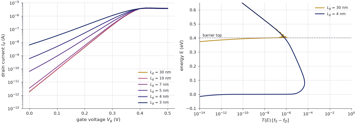
Down to 10 nm the swing stays at the thermal limit. At 7 nm it rises to 62 mV/dec, at 5 nm to 86 mV/dec and at 3 nm to 143 mV/dec, and the off current at \(V_g = 0\) grows by more than three orders of magnitude. The energy-resolved current on the right shows why: for the 30 nm channel essentially everything flows above the barrier top, for the 4 nm channel 99.7 % of the current tunnels through it. This source-to-drain tunneling sets one of the limits of scaling, and it cannot be described by a band diagram and a Fermi function alone: it needs quantum mechanics, and — as Lecture 1.3 argues — the right band structure inside the barrier.
4. A three-dimensional device: a gate-all-around nanowire#
The model above imposes the barrier. In a real transistor the barrier is set by electrostatics:
the gate, the doping and the electrons themselves, through Poisson's equation. open-nemo's
GateAllAroundWire solves this self-consistently for a silicon nanowire wrapped by its gate:
a 2 nm diameter [100] wire, 1 nm of oxide, an 8 nm gate and 8 nm source and drain extensions doped
\(10^{20}\) cm⁻³, with the cross-section's subbands of two valley pairs (four each) carrying
ballistic current along the wire (the mode-space approach of
the gate-all-around nanowire FET notebook).
Six gate voltages at \(V_d\) = 0.5 V take about half a minute.
Code
wire = nemo.devices.nanowire.GateAllAroundWire(diameter=2.0, t_ox=1.0, gate_length=8.0,
                                               sd_length=8.0, donors=1e20, orientation=100,
                                               valleys=2, modes=4)
vg_w = np.linspace(0.0, 0.5, 6)
res = wire.solve(vg_w, drain_voltage=0.5)
iw = np.asarray(res["current"])
print("V_g (V)   I_d (A)     iterations")
for v, i, n in zip(vg_w, iw, res["iterations"]):
    print(f"{v:6.2f}   {i:10.3e}   {n:4d}")
print(f"swing between 0 and 0.1 V: {1e3 * 0.1 / np.log10(iw[1] / iw[0]):.1f} mV/dec, "
      f"between 0.1 and 0.2 V: {1e3 * 0.1 / np.log10(iw[2] / iw[1]):.1f} mV/dec")

fig, (ax1, ax2) = plt.subplots(1, 2, figsize=(11, 4))
for c, k in zip(style.sweep(len(vg_w)), range(len(vg_w))):
    ax1.plot(res["z"], res["subbands"][k][0][0], color=c, label=f"$V_g$ = {vg_w[k]:.1f} V")
ax1.axhline(0.0, color=style.CONTEXT, ls="--", lw=1)
ax1.set(xlabel="position along the wire z (nm)", ylabel="lowest subband (eV, source $E_F$ = 0)")
ax1.legend(fontsize=8)
ax2.semilogy(vg_w, iw, "o-", color=style.OPEN_NEMO, label="open-nemo, self-consistent")
ax2.semilogy(vg_w, iw[0] * 10 ** (vg_w / (KB * 300 * np.log(10))), color=style.REFERENCE, ls="--",
             lw=1, label="60 mV/dec")
ax2.set(xlabel="gate voltage $V_g$ (V)", ylabel="drain current $I_d$ (A)")
ax2.legend(fontsize=8)
fig.tight_layout()
V_g (V)   I_d (A)     iterations
  0.00    2.226e-12      5
  0.10    9.056e-11      5
  0.20    3.499e-09      4
  0.30    1.056e-07      4
  0.40    1.292e-06      5
  0.50    5.078e-06     10
swing between 0 and 0.1 V: 62.1 mV/dec, between 0.1 and 0.2 V: 63.0 mV/dec
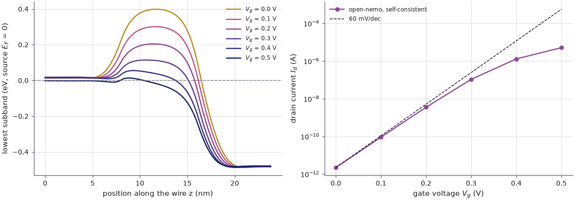
The self-consistent wire reproduces the textbook picture. The lowest subband along the wire (left) is the band diagram of slide 4: a barrier under the gate that the gate voltage pulls down, with the drain side 0.5 V lower. The current (right) rises from about 2 pA to 5 µA, close to the curve in the slide's animation, with a swing of 62 mV/dec between 0 and 0.1 V: the gate wrapped around a 2 nm wire controls the channel almost perfectly (\(\alpha \approx 59.5/62.1 = 0.96\)). Above 0.3 V the channel fills with electrons, their charge screens the gate, and the current bends over. Note that in a flat potential the lowest subband of this 2 nm wire lies 0.42 eV above the bulk band edge (see the nanowire notebook): confinement is not a small correction here.
5. Beyond the transistor: optical interactions#
The last picture leaves the transistor. A thin GaAs layer between AlGaAs barriers confines electrons in the conduction band and holes in the valence band. An electron dropping from the first conduction-band level to the first valence-band level emits a photon of energy
where \(E_{e1}\) and \(E_{h1}\) are the confinement energies measured from the band edges. The questions the slide adds — the valence band, light emission and absorption, electron–electron and electron–phonon interactions — are all needed for lasers, LEDs and photodetectors.
The levels come from closed effective-mass boxes: the well between two 10 nm barriers, with the offsets of open-nemo's material registry for Al${0.3}$Ga${0.7}$As on GaAs, the electron masses of the two materials, and the heavy-hole mass along [001], \(m_{hh} = m_0/(\gamma_1 - 2\gamma_2)\) from the GaAs Luttinger parameters (used in both layers, a simplification).
Code
props = nemo.structures.properties
eg_w, eg_b = props.value("GaAs", "band_gap"), props.value("AlGaAs", "band_gap", x=0.3)
dev_v = props.value("AlGaAs", "valence_band_offset", x=0.3) - props.value("GaAs", "valence_band_offset")
dec = (eg_b - eg_w) + dev_v                     # conduction-band offset (eV)
dhv = -dev_v                                    # valence-band offset, as a barrier for holes (eV)
m_e, m_eb = effective_mass("GaAs").mass, effective_mass("AlGaAs", x=0.3).mass
m_hh = 1.0 / (props.value("GaAs", "luttinger_gamma1") - 2 * props.value("GaAs", "luttinger_gamma2"))
print(f"E_g(GaAs) = {eg_w:.4f} eV, ΔE_c = {dec:.3f} eV, ΔE_v = {dhv:.3f} eV, "
      f"m_e = {m_e:.3f}/{m_eb:.4f}, m_hh = {m_hh:.3f} m0")


def lowest_level(width, m_well, m_bar, offset, barrier=10.0):
    w = EffectiveMassMaterial("well", m_well, 12.9)
    b = EffectiveMassMaterial("barrier", m_bar, 12.9, conduction_band_edge=offset)
    box = nemo.Heterostructure1D([nemo.Layer(b, barrier), nemo.Layer(w, width), nemo.Layer(b, barrier)],
                                 spacing=0.05)
    h = box.hamiltonian.sparse.matrices[0]
    e = eigh_tridiagonal(h.diagonal().real, h.diagonal(1).real, select="i", select_range=(0, 0))[0]
    return e[0]


print("\n L (nm)   E_e1 (meV)  [inf. well]   E_h1 (meV)  [inf. well]   ħω (eV)   λ (nm)")
widths = np.array([3.0, 5.0, 8.0, 12.0, 20.0])
hw = []
for L in widths:
    ee, eh = lowest_level(L, m_e, m_eb, dec), lowest_level(L, m_hh, m_hh, dhv)
    inf_e, inf_h = H2M0 * np.pi**2 / (m_e * L**2), H2M0 * np.pi**2 / (m_hh * L**2)
    hw.append(eg_w + ee + eh)
    print(f"{L:6.0f}   {1e3 * ee:9.1f}  [{1e3 * inf_e:7.1f}]   {1e3 * eh:9.1f}  [{1e3 * inf_h:7.1f}]   "
          f"{hw[-1]:7.3f}   {1239.84 / hw[-1]:6.0f}")
print(f"bulk GaAs: {eg_w:.3f} eV, {1239.84 / eg_w:.0f} nm")
E_g(GaAs) = 1.4225 eV, ΔE_c = 0.259 eV, ΔE_v = 0.159 eV, m_e = 0.067/0.0919, m_hh = 0.350 m0

 L (nm)   E_e1 (meV)  [inf. well]   E_h1 (meV)  [inf. well]   ħω (eV)   λ (nm)
     3       128.2  [  623.6]        47.6  [  119.5]     1.598      776
     5        77.0  [  224.5]        23.9  [   43.0]     1.523      814
     8        42.4  [   87.7]        11.5  [   16.8]     1.476      840
    12        23.4  [   39.0]         5.8  [    7.5]     1.452      854
    20        10.2  [   14.0]         2.3  [    2.7]     1.435      864
bulk GaAs: 1.422 eV, 872 nm
A 20 nm well emits 13 meV above bulk GaAs (872 nm); an 8 nm well emits at 1.48 eV (840 nm), a 3 nm well at 1.60 eV (776 nm), close to the visible red. The emission color is set by the thickness of a layer, a few nanometres, through confinement. The infinite-well formula \(\hbar^2\pi^2/2m^*L^2\) in brackets overestimates the levels badly once the well is narrow, because the wave function leaks into the barriers; a real design also needs the valence-band mixing that a single heavy-hole mass ignores (the eight-band k·p heterostructures and quantum-well optics notebooks include it).
6. A thousand questions, and where this course answers them#
The slides end with the learning outcomes: explain the working principles of these devices, explain the physical processes in them, and relate their performance to materials and design criteria. The list of questions maps onto the course. The conduction and valence bands, effective masses, non-parabolicity and the crystal come with band structure (Lecture 1.3 and the tight-binding sections); doping, density of states and the Fermi distribution with the electrostatics of devices (Lecture 1.4); confinement and tunneling with the open-system and resonant-tunneling sections; geometry and strain with the nanowire and ultra-thin-body material; scattering by electrons and phonons with the transport sections and Lecture 2.
Summary#
- A one-dimensional barrier model with ballistic transmission reproduces the textbook band diagram and the \(\log I_d\)–\(V_g\) curve; a single mode saturates near \((2q/h)k_BT\ln(1+e^{\mu_S/k_BT})\) = 4.1 µA.
- Below threshold only the Fermi tail crosses the barrier, so the swing is \(S = (k_BT/q)\ln 10/\alpha\): 59.3 mV/dec computed against 59.5 at 300 K, 15.3 at 77 K, 74.7 for \(\alpha\) = 0.8.
- Channels shorter than about 7 nm let electrons tunnel under the barrier top: the swing rises to 86 mV/dec at 5 nm and 143 mV/dec at 3 nm.
- A self-consistent 2 nm gate-all-around silicon wire gives 62 mV/dec and a current from about 2 pA to 5 µA between 0 and 0.5 V.
- In a GaAs/Al${0.3}$Ga${0.7}$As quantum well the photon energy moves from 1.44 eV (20 nm) to 1.60 eV (3 nm) by confinement alone.
Exercises#
- Repeat the swing calculation at 4 K. What limits the swing of the 30 nm channel there, and what would you have to change in the model to recover \(k_BT\ln10/q\)?
- Replace the transverse mass \(0.19\,m_0\) by the longitudinal mass \(0.916\,m_0\) (the Δ valleys whose heavy direction lies along the channel). How does the swing of the 4 nm channel change, and why?
- Make the gate coupling depend on the channel length, e.g. \(\alpha = 1 - e^{-L_g/2\lambda}\) with a natural length \(\lambda\) = 2 nm, and combine it with the tunneling of Section 3. Which effect dominates at 5 nm?
- Find the well width at which the GaAs quantum well emits at 800 nm.
Further reading#
- Gate-all-around nanowire FET
- Gate geometry and scaling
- Wire tunnel FETs, which beat 60 mV/dec by filtering the Fermi tail with a band-to-band tunnel junction
- Quantum-well optics
- Lecture 1.3: band structure in nanoelectronics and Lecture 1.4: PN junction to device scaling
- R. F. Pierret, Semiconductor Device Fundamentals (Addison-Wesley, 1996).
- M. Lundstrom and J. Guo, Nanoscale Transistors: Device Physics, Modeling and Simulation (Springer, 2006).
- The animation on slide 7: en.wikipedia.org/wiki/File:Threshold_formation_nowatermark.gif