Lecture 11.4

RTDs with quantum charge self-consistency (Hartree model)

In the lecture

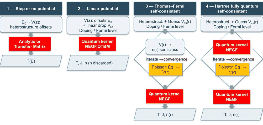
four levels of approximation for the potential of an RTD: no potential, a linear drop, a Thomas–Fermi self-consistent potential with one quantum pass, and Hartree self-consistency with the quantum kernel inside the loop
semiclassical against quantum charge: smooth profiles, charge in the barriers, a rounded well charge, no spike at the interface; the relaxation model leaves the quantum charge in the reservoirs at about 80% of the semiclassical one
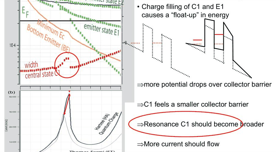
how quantum charge in the well makes the central resonance float up and resist being pulled down: the I–V is stretched and linearised, and the peak moves to a higher voltage
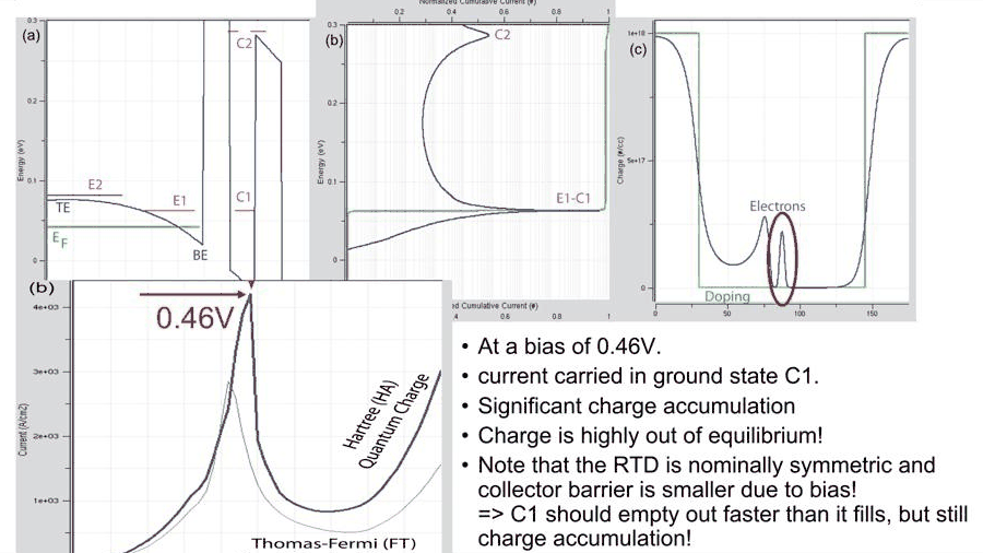
charge accumulation at the peak even in a symmetric RTD, and the valley where the well is empty
why the peak current increases: more potential drops over the collector barrier, so C1 broadens

In this notebook

takes the realistic-doping RTD of lectures 11.2–11.3 and compares the band profiles and I–V curves of a linear drop, the Thomas–Fermi model (nemo.thomas_fermi_iv) and the Hartree model (nemo.hartree_iv); it computes the quantum charge on the Thomas–Fermi potential with ReservoirTransport, traces the central resonance energy and width and the sheet charge in the well against bias, splits the valley current, and varies the region where the charge is computed quantum mechanically.

Run the notebookEvery number and figure on this page comes from it. Change it, rerun it, take it further.

Download .ipynb View on GitHub

Run it on your own machine

The notebook needs open-nemo (Python ≥ 3.10 and a C++20 compiler; BLAS/LAPACK).

git clone https://github.com/denphi/open-nemo.git && cd open-nemo
python3 -m venv .venv && source .venv/bin/activate
pip install -e ".[notebooks]"
jupyter lab From_Atoms_to_Devices/06_resonant_tunneling_diodes/11_4_hartree_self_consistency.ipynb

Code8 lines · cell 1

import numpy as np
import matplotlib.pyplot as plt
import opennemo as nemo
from opennemo.visualization import style

style.use(notebook=True)
H2M0 = nemo.core.units.HBAR2_2M0          # ħ²/2m₀ = 0.0381 eV nm²
EM = nemo.structures.materials.EffectiveMassMaterial

1. Four levels of approximation#

The lectures of this section climb a ladder of models for the electrostatic potential $V(z)$ of an RTD:

level	potential	charge	what it gives
1	band offsets only (step potential)	none	$T(E)$, analytically or with transfer matrices
2	offsets plus an assumed linear drop	computed but discarded	$T(E)$, $J(E)$, $J$ (lecture 11.1)
3	Thomas–Fermi self-consistent	semiclassical $n(z)$ in the Poisson loop; one quantum (NEGF) pass afterwards	band bending, notch states, injection from quasi-bound emitter states (lectures 11.2–11.3)
4	Hartree self-consistent	quantum $n(z)$ from the NEGF kernel inside the Poisson loop	no unphysical charge spikes, non-equilibrium charge accumulation in the well

Level 3 is very fast and already gives a realistic potential, but the charge it puts back into Poisson's equation is semiclassical: the charge of the well, which is out of equilibrium and has no Fermi level, does not act back on the potential. Level 4 iterates the quantum charge with the potential until both agree. It is still a mean-field (effective potential) model: the electron–electron interaction of discrete charges is not included.

Slide 7: the four levels of approximation, from step potential to Hartree self-consistency — Slide 7. The four levels of approximation. Level 1: band offsets, analytic or transfer-matrix $T(E)$. Level 2: offsets plus a linear drop, quantum kernel (NEGF or QTBM). Level 3: Thomas–Fermi self-consistent potential, then a quantum kernel. Level 4: the quantum kernel inside the Poisson loop (Hartree).

The device is the one of lectures 11.2 and 11.3: 30 nm GaAs contacts doped to $10^{18}$ cm$^{-3}$, 50 nm spacers at $10^{15}$ cm$^{-3}$, and 4 nm Al${0.3}$Ga${0.7}$As barriers around a 5 nm GaAs well, at 300 K. All self-consistent calculations use NEMO's reservoir relaxation of 6.6 meV. In nemo.hartree_iv the quantum (NEGF) charge is used on the sites given by quantum_charge, counted from the edges of the double barrier; (-200, 200) covers both 50 nm spacers, including the emitter notch, and the Thomas–Fermi charge is kept only in the doped contacts.

Code26 lines · cell 5

from opennemo.solvers.reservoir import ReservoirTransport, reservoir_transmission

x_al = 0.3
gaas = EM("GaAs", 0.067, 12.9, conduction_band_edge=0.0)
algaas = EM("Al0.3Ga0.7As", 0.067 + 0.083 * x_al, 12.9 - 2.84 * x_al, conduction_band_edge=0.324)
layers = [
    nemo.Layer(gaas, 30, donors=1e18, name="emitter contact"),
    nemo.Layer(gaas, 50, donors=1e15, name="emitter spacer"),
    nemo.Layer(algaas, 4, name="barrier"),
    nemo.Layer(gaas, 5, name="well"),
    nemo.Layer(algaas, 4, name="barrier"),
    nemo.Layer(gaas, 50, donors=1e15, name="collector spacer"),
    nemo.Layer(gaas, 30, donors=1e18, name="collector contact"),
]
rtd = nemo.Heterostructure1D(layers, spacing=0.25, terminal_layers=(2, 2))
x, XB1 = rtd.x, 80.0
well = (x > XB1 + 4) & (x < XB1 + 9)
T = 300
V = np.round(np.arange(0.0, 0.8001, 0.02), 3)
tf = nemo.thomas_fermi_iv(rtd, V, T, charge="all")
hartree = nemo.hartree_iv(rtd, V, T, quantum_charge=(-200, 200))
EF = float(np.atleast_1d(tf["mu_left"])[0])
print(
    f"Hartree: all biases converged: {bool(np.all(hartree['converged']))}, "
    f"iterations per bias {int(np.min(hartree['iterations']))}-{int(np.max(hartree['iterations']))}"
)

Hartree: all biases converged: True, iterations per bias 2-7

For level 2 the same device gets the linear drop of lecture 11.1: flat bands everywhere outside the double barrier (no hump, no notch) and a linear drop across barriers and well only; the ballistic current is computed with nemo.Transport.

Code22 lines · cell 7

tr = nemo.Transport(rtd.hamiltonian)
ramp = np.clip((x - XB1) / 13.0, 0, 1)  # drop across barrier, well, barrier (80 to 93 nm)
kT = 8.617e-5 * T


def linear_drop_current(v):
    u = -v * ramp
    r = nemo.resonances(rtd, potential=u, emin=-v, emax=0.4)
    seeds = [e + w * np.linspace(-12, 12, 121) for e, w in zip(r["energy"], r["width"])]
    E = np.unique(np.concatenate([np.linspace(1e-5, EF + 15 * kT, 1500)] + seeds))
    E = E[(E > 0) & (E < EF + 15 * kT)]
    return rtd.current_density(E, tr.transmission(E, potential=u), EF, EF - v, T)


J_lin = np.array([linear_drop_current(v) for v in V])
i40 = int(np.argmin(abs(V - 0.4)))
fig, ax = plt.subplots(figsize=(7, 3.8))
ax.plot(x, rtd.band_edge - 0.4 * ramp, color=style.CONTEXT, label="2: linear drop")
ax.plot(x, rtd.band_edge + tf["potential"][i40], **style.series("reference"), label="3: Thomas–Fermi")
ax.plot(x, rtd.band_edge + hartree["potential"][i40], **style.series(lw=2), label="4: Hartree")
ax.set(xlabel="Position (nm)", ylabel="Energy (eV)", ylim=(-0.45, 0.45), title="Conduction band at 0.40 V")
ax.legend();

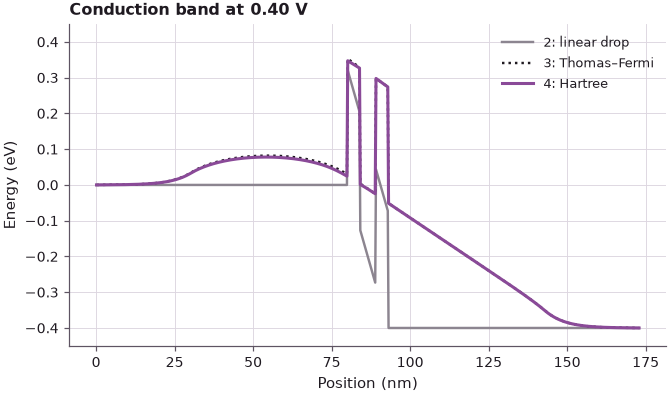
Figure computed by the notebook with open-nemo

The Thomas–Fermi and Hartree potentials are close to each other and both very different from the linear drop: the emitter hump, the notch, and the long linear drop through the depleted collector spacer are features of the electrostatics, not of the quantum treatment. The lecture's conclusion is the same: the semiclassical potential is a much better approximation to the Hartree one than any assumed linear drop. The differences that remain are in the double barrier itself, and they matter for the current.

2. Semiclassical against quantum charge#

Before iterating, it is instructive to compute the quantum charge once on the Thomas–Fermi potential. ReservoirTransport(...).electron_density integrates the NEGF spectral densities injected from both sides with their Fermi functions, including the broadened states of the reservoirs. The energy grid is seeded with points across every resonance.

Code22 lines · cell 10

rt = ReservoirTransport(rtd, eta=0.0066, decay=0.0066)
RES = (0.0066, 0.0066, "exponential", (-1, 0))
regions = {
    "emitter contact": (5, 25),
    "emitter spacer": (40, 70),
    "notch": (70, 79.9),
    "well": (84.5, 88.5),
    "collector spacer": (100, 140),
    "collector contact": (150, 170),
}
nq = {}
for v in (0.0, 0.4):
    i = int(np.argmin(abs(V - v)))
    u = tf["potential"][i]
    r = nemo.resonances(rtd, potential=u, confinement_region=(-160, 0), emax=0.3, reservoir=RES)
    seed = np.concatenate([e + w * np.linspace(-5, 5, 21) for e, w in zip(r["energy"], r["width"])])
    nq[v] = rt.electron_density(u, EF, EF - v, T, seed=seed)
    ratios = []
    for name, (a, b) in regions.items():
        m = (x > a) & (x < b)
        ratios.append(f"{name} {nq[v][m].sum() / tf['electron_density'][i][m].sum():.2f}")
    print(f"{v:.1f} V, quantum/semiclassical charge: " + ", ".join(ratios))

0.0 V, quantum/semiclassical charge: emitter contact 0.84, emitter spacer 0.87, notch 0.67, well 0.13, collector spacer 0.89, collector contact 0.84
0.4 V, quantum/semiclassical charge: emitter contact 0.84, emitter spacer 0.86, notch 0.60, well 53.80, collector spacer 1.00, collector contact 0.84

Code12 lines · cell 11

fig, axes = plt.subplots(1, 2, figsize=(11, 3.8), sharey=True)
for ax, v in zip(axes, (0.0, 0.4)):
    i = int(np.argmin(abs(V - v)))
    ax.semilogy(x, tf["electron_density"][i], **style.series("reference"), label="semiclassical (Thomas–Fermi)")
    ax.semilogy(x, nq[v], **style.series(lw=2), label="quantum (NEGF, one pass)")
    ax.semilogy(x, rtd.donors, color=style.CONTEXT, lw=1, label="donors")
    ax.set(
        xlabel="Position (nm)", title=f"{v:.1f} V, Thomas–Fermi potential", ylim=(1e13, 3e18), xlim=(40, 140)
    )
axes[0].set_ylabel("Electron density (cm$^{-3}$)")
axes[0].legend(fontsize=8, loc="lower left")
fig.tight_layout();

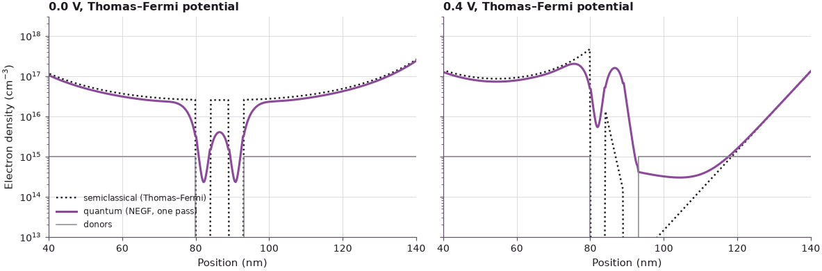
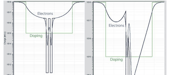
Slide 8: semiclassical and quantum charge of the RTD at zero bias and under bias — Slide 8. Semiclassical (black, with sharp steps) and quantum (blue) electron density with the doping (green), in equilibrium (left) and under bias (right). The quantum charge is smooth, enters the barriers and is rounded in the well.

The quantum charge is smooth: it leaks into the barriers by tunnelling, it has the rounded shape of the resonance in the well, and it vanishes towards the interface of the notch instead of piling up in a spike. Two differences are quantitative:

In the reservoirs the quantum charge is only about 84% of the semiclassical one, close to the lecture's "about 80%". The relaxation $-i\eta$ broadens and partly removes the density of states near the band edge; the lecture calls this a "non-conserving density of states reduction". It is one reason the charge has to be computed self-consistently with the relaxation switched on.
Under bias the well holds far more quantum charge than the Thomas–Fermi model puts there, because the well is filled from the emitter and has no Fermi level of its own: its charge is out of equilibrium.

At zero bias the well charge is small in both models, and the relaxation has no effect on it, since there is no optical potential in the central region.

3. The I–V with quantum charge self-consistency#

Code24 lines · cell 15

J_tf, J_h = tf["current_density"], hartree["current_density"]


def first_peak(J):
    return next(i for i in range(1, len(J) - 1) if J[i] >= J[i - 1] and J[i] > J[i + 1])


for name, J in (
    ("linear drop (ballistic)", J_lin),
    ("Thomas–Fermi + relaxation", J_tf),
    ("Hartree + relaxation", J_h),
):
    k = first_peak(J)
    print(
        f"{name:26s}: first peak {J[k]:6.0f} A/cm^2 at {V[k]:.2f} V, valley {J[k:k + 15].min():6.0f} A/cm^2"
    )

fig, ax = plt.subplots(figsize=(6.5, 4))
ax.plot(V, J_lin, color=style.CONTEXT, lw=1.5, ls="--", label="2: linear drop")
ax.set_ylim(0, 1.6 * J_h.max())
ax.plot(V, J_tf, **style.series("reference"), label="3: Thomas–Fermi")
ax.plot(V, J_h, **style.series(lw=2), label="4: Hartree")
ax.set(xlabel="Bias (V)", ylabel="Current density (A/cm²)", title="Three potential models, 300 K")
ax.legend();

linear drop (ballistic)   : first peak  11864 A/cm^2 at 0.12 V, valley    773 A/cm^2
Thomas–Fermi + relaxation : first peak   6786 A/cm^2 at 0.42 V, valley   1557 A/cm^2
Hartree + relaxation      : first peak   9790 A/cm^2 at 0.50 V, valley   2022 A/cm^2

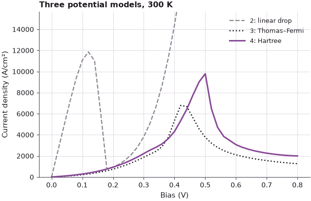
The Hartree I–V peaks at 0.50 V with 9790 A/cm$^2$, against 0.42 V and 6786 A/cm$^2$ for Thomas–Fermi: a higher voltage and a higher current, as in the lecture, and its rising branch is straighter (the voltage axis is stretched). The linear drop, which ignores the emitter hump and the voltage absorbed in the spacers, puts the first peak at 0.12 V, and beyond 0.3 V its current rises steeply as the barriers themselves are pulled down. To see where the Hartree changes come from, the next cell follows the central resonance C1 and the sheet charge in the well.

Code23 lines · cell 17

def c1(pot):
    """Energy and width of C1, with the reservoir relaxation (which broadens the emitter states)."""
    r = nemo.resonances(rtd, potential=pot, emax=0.3, emin=float(np.min(rtd.band_edge + pot)), reservoir=RES)
    k = np.flatnonzero((r["x0"] > XB1 + 3) & (r["x0"] < XB1 + 10) & (r["width"] < 3e-3))[0]
    return r["energy"][k], r["width"][k]


trace = {
    name: np.array([c1(res["potential"][i]) for i in range(len(V))])
    for name, res in (("Thomas–Fermi", tf), ("Hartree", hartree))
}
sheet = {
    name: res["electron_density"][:, well].sum(1) * rtd.spacing * 1e-7
    for name, res in (("Thomas–Fermi", tf), ("Hartree", hartree))
}
kh = int(np.argmax(J_h))
for name in trace:
    kw = int(np.argmax(trace[name][:, 1]))
    print(
        f"{name:13s}: C1 at 0.48 V {1e3 * trace[name][V == 0.48, 0][0]:.1f} meV; C1 width 0 V "
        f"{1e3 * trace[name][0, 1]:.2f} meV, largest {1e3 * trace[name][kw, 1]:.2f} meV at {V[kw]:.2f} V; "
        f"well sheet density at {V[kh]:.2f} V {sheet[name][kh]:.2g} cm^-2"
    )

Thomas–Fermi : C1 at 0.48 V 56.3 meV; C1 width 0 V 0.41 meV, largest 0.56 meV at 0.42 V; well sheet density at 0.50 V 7.4e+08 cm^-2
Hartree      : C1 at 0.48 V 62.7 meV; C1 width 0 V 0.41 meV, largest 0.60 meV at 0.48 V; well sheet density at 0.50 V 1e+11 cm^-2

Code13 lines · cell 18

fig, axes = plt.subplots(1, 3, figsize=(12, 3.6))
for name, c in (("Thomas–Fermi", style.REFERENCE), ("Hartree", style.OPEN_NEMO)):
    axes[0].plot(V, trace[name][:, 0], color=c, lw=2, label=name)
    axes[1].plot(V, 1e3 * trace[name][:, 1], color=c, lw=2, label=name)
    axes[2].semilogy(V, sheet[name], color=c, lw=2, label=name)
axes[0].axhline(EF, color=style.CONTEXT, ls=":", label="$E_F$ (emitter)")
axes[0].set(xlabel="Bias (V)", ylabel="Energy (eV)", title="Central resonance C1")
axes[1].set(xlabel="Bias (V)", ylabel="Width (meV)", title="Width of C1")
axes[2].set(xlabel="Bias (V)", ylabel="Sheet density (cm$^{-2}$)", title="Electrons in the well")
for a in axes:
    a.axvline(V[kh], color="C3", lw=0.8, ls="--")
axes[0].legend(fontsize=8)
fig.tight_layout();

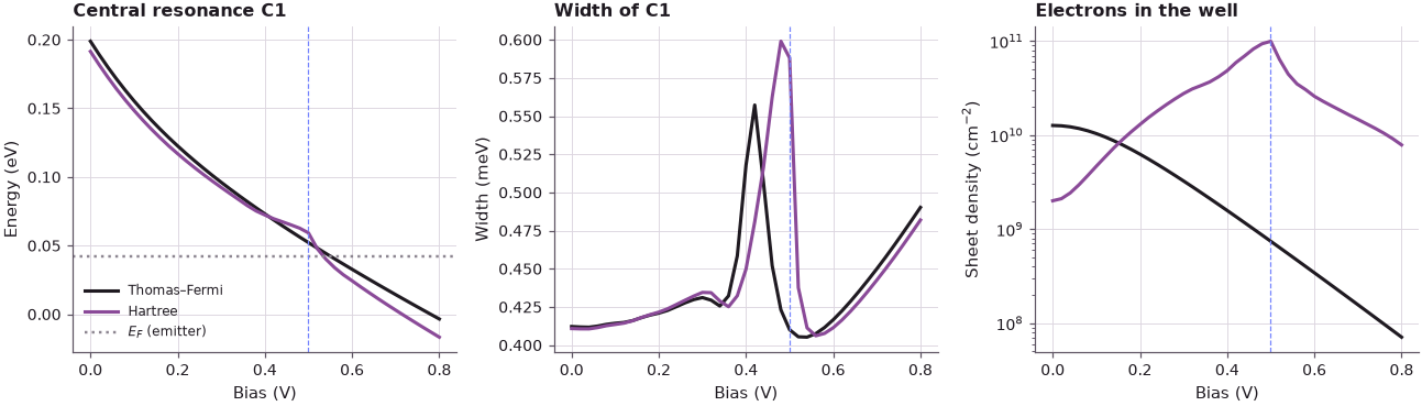
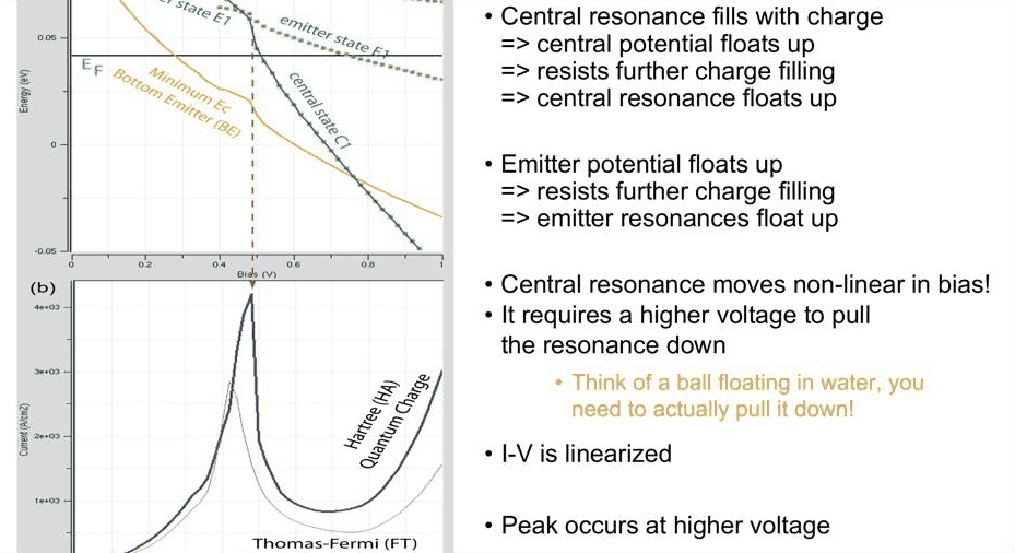
Slide 12: resonance traces and I–V with quantum charge self-consistency — Slide 12. (a) Traces of the central resonance, emitter states and emitter band edges with quantum charge self-consistency; (b) Hartree I–V (blue) against the Thomas–Fermi I–V (thin): the resonance floats up, a higher voltage is needed to pull it down, the I–V is linearised and the peak occurs at a higher voltage.

The lecturer's picture is a ball floating in water. As C1 comes down into the supply, it fills with electrons. That charge raises the potential of the well, which lifts C1 back up and resists further filling; the emitter charge does the same to the emitter states. One has to "pull harder" to bring the resonance down, so C1 no longer falls almost linearly, and the current keeps rising until C1 finally disengages from the emitter supply. In the Thomas–Fermi model the well charge is the small equilibrium-like charge of a local Fermi level, so C1 falls freely.

The traces show this in numbers. At 0.48 V the Hartree C1 is at 62.7 meV, 6 meV above its Thomas–Fermi position, and it stays nearly level between 0.4 and 0.5 V before it drops. The charge in the well peaks with the current: at 0.50 V the Hartree well holds $10^{11}$ electrons per cm$^2$, more than a hundred times the Thomas–Fermi value of $7.4\times10^{8}$ cm$^{-2}$, although the RTD is nominally symmetric. Under bias the collector barrier is effectively lower than the emitter barrier, so electrons leave the well faster than they enter, but the entry rate is high enough to pile up charge. This charge is highly out of equilibrium: it is charge in transit.

Slide 13: charge accumulation at the current peak when C1 is aligned with E1 — Slide 13. At the peak (0.46 V in the lecture) C1 is aligned with the emitter state E1, the current flows through C1, and the well holds a large non-equilibrium charge (circled), even though the RTD is nominally symmetric.

4. Why the peak current increases#

Stretching alone would only move the peak. The peak is also higher, and the width trace shows why. The well charge lifts the potential of the well, so more potential drops over the collector barrier; C1 sees a steeper, effectively thinner triangular collector barrier and its width grows in the bias range where the well is charged: in the Hartree potential it reaches 0.60 meV at 0.48 V, against 0.41 meV at zero bias (the Thomas–Fermi trace has a smaller bump, 0.56 meV at 0.42 V, where C1 crosses the broadened E1). A broader filter passes more current. Once the well empties beyond the peak, the width returns to the uncharged value and C1 again falls almost linearly.

Slide 16: why the peak current increases, with the C1 width rising in the charged bias range — Slide 16. Charge in C1 and E1 makes the potential float up, more potential drops over the collector barrier, C1 sees a thinner collector barrier and becomes broader (circled width trace), so more current flows.

5. The valley: an empty well and current below the band edge#

In the valley at 0.76 V the lecture finds C1 aligned with the bottom of the emitter. There should be no supply at that energy, the well is empty, yet about 25% of the current still flows through C1: the relaxation of the reservoirs decays exponentially below the band edge (an Urbach tail) and injects some electrons there. The cell repeats this analysis on the Hartree potential.

Code20 lines · cell 25

i76 = int(np.argmin(abs(V - 0.76)))
u = hartree["potential"][i76]
e_c1, g_c1 = c1(u)
bottom = (rtd.band_edge + u)[x < XB1][-1]
E = np.unique(
    np.concatenate([np.linspace(-0.15, EF + 15 * kT, 6000), e_c1 + g_c1 * np.linspace(-20, 20, 201)])
)
t = reservoir_transmission(rtd, u)(E)
Je = rtd.current_spectrum(E, t, EF, EF - V[i76], T)
J = rtd.current_density(E, t, EF, EF - V[i76], T)
cum = np.concatenate([[0], np.cumsum(0.5 * (Je[1:] + Je[:-1]) * np.diff(E))]) / J
at = lambda e: cum[np.argmin(abs(E - e))]
print(
    f"{V[i76]:.2f} V: J = {J:.0f} A/cm^2 (hartree_iv: {J_h[i76]:.0f}); C1 at {1e3 * e_c1:.1f} meV, "
    f"emitter bottom at {1e3 * bottom:.1f} meV"
)
print(
    f"share within ±3 meV of C1: {100 * (at(e_c1 + 3e-3) - at(e_c1 - 3e-3)):.0f}%; "
    f"well sheet density {sheet['Hartree'][i76]:.2g} cm^-2 (peak: {sheet['Hartree'][kh]:.2g})"
)

0.76 V: J = 2056 A/cm^2 (hartree_iv: 2059); C1 at -8.9 meV, emitter bottom at -20.8 meV
share within ±3 meV of C1: 57%; well sheet density 1e+10 cm^-2 (peak: 1e+11)

The well holds $10^{10}$ cm$^{-2}$, an order of magnitude less than at the peak, and C1 (at $-8.9$ meV) is only 12 meV above the bottom of the emitter notch. Still 57% of the current passes through C1, more than the 25% of the lecture's device, fed by the broadened emitter states and their tails. Valley currents are the hardest quantity to predict, because they depend on such details of the contact model.

6. Exploration: how much of the device needs quantum charge?#

NEMO-1D's default computes the quantum charge only in the double barrier and 16–17 monolayers (about 4 nm) on each side, with Thomas–Fermi charge everywhere else, including most of the notch. The cell compares that choice with the quantum charge over both spacers used above.

Code11 lines · cell 28

h_small = nemo.hartree_iv(rtd, V, T)  # quantum_charge=(-17, 16), NEMO-1D's default
J_s = h_small["current_density"]
for name, J in (("quantum charge over the spacers", J_h), ("NEMO-1D default (-17, 16)", J_s)):
    k = int(np.argmax(J))
    print(f"{name:32s}: peak {J[k]:6.0f} A/cm^2 at {V[k]:.2f} V")
fig, ax = plt.subplots(figsize=(6, 3.6))
ax.plot(V, J_tf, **style.series("reference"), label="Thomas–Fermi")
ax.plot(V, J_s, **style.series("nemo-family", lw=2), label="Hartree, quantum charge ±4 nm")
ax.plot(V, J_h, **style.series(lw=2), label="Hartree, quantum charge over the spacers")
ax.set(xlabel="Bias (V)", ylabel="Current density (A/cm²)", title="Where the charge is quantum")
ax.legend(fontsize=8);

quantum charge over the spacers : peak   9790 A/cm^2 at 0.50 V
NEMO-1D default (-17, 16)       : peak   8787 A/cm^2 at 0.48 V

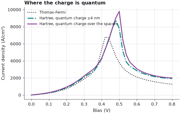
Most of the change from Thomas–Fermi to Hartree comes from the quantum charge in and next to the well (peak 8787 A/cm$^2$ at 0.48 V with NEMO-1D's default); treating the emitter notch quantum mechanically as well raises the peak further, to 9790 A/cm$^2$ at 0.50 V, since the semiclassical notch charge, with its spike, overestimates the screening in front of the barrier.

Summary#

Four levels of approximation: no potential, a linear drop, Thomas–Fermi self-consistency with one quantum pass, and Hartree self-consistency with the quantum charge inside the loop.
Semiclassical and quantum charge differ at interfaces and inside the RTD. The quantum charge is smooth, tunnels into the barriers and has no spike; with reservoir relaxation it is about 80–85% of the semiclassical charge in the contacts, and in the biased well it is a large non-equilibrium charge.
The Thomas–Fermi potential is a far better approximation to the Hartree potential than a linear drop.
Hartree self-consistency makes the charged resonance float up: the voltage axis is stretched, the I–V linearised, and the peak moves to higher bias. The peak current rises because more potential drops over the collector barrier and C1 broadens.
Even a symmetric RTD accumulates charge at the current peak; in the valley the well is empty and part of the current is fed by the relaxation tails below the band edge.

Exercises#

Run nemo.hartree_iv with exchange_correlation=True. How large is the exchange–correlation potential in the well at the peak, and how does it move the peak?
Compute the Hartree I–V at 77 K with initial_guess="previous" for an up-sweep and a down-sweep (pass the biases in reverse order). Is there hysteresis around the peak?
Plot the Hartree potential in the well at 0, 0.3 V and the peak bias, measured from the linear drop between the two barrier edges. How many meV does the well charge lift C1 at the peak?
Repeat the comparison of section 3 with 7 nm barriers. Is the stretching larger or smaller, and why?

level	potential	charge	what it gives
1	band offsets only (step potential)	none	\(T(E)\), analytically or with transfer matrices
2	offsets plus an assumed linear drop	computed but discarded	\(T(E)\), \(J(E)\), \(J\) (lecture 11.1)
3	Thomas–Fermi self-consistent	semiclassical \(n(z)\) in the Poisson loop; one quantum (NEGF) pass afterwards	band bending, notch states, injection from quasi-bound emitter states (lectures 11.2–11.3)
4	Hartree self-consistent	quantum \(n(z)\) from the NEGF kernel inside the Poisson loop	no unphysical charge spikes, non-equilibrium charge accumulation in the well