Lecture 10.4

Introduction to transport — sequential versus coherent tunneling

In the lecture

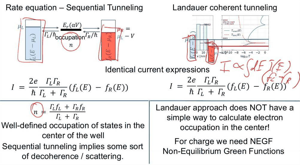
the rate equation of sequential tunneling (Lecture 10.2) and the Landauer formula of coherent tunneling (Lecture 10.3) give identical current expressions for a narrow, isolated resonance
the sequential picture has a well-defined occupation of the state in the well; it implies some decoherence or scattering
the Landauer approach has no expression for the charge in the device; for the charge one needs non-equilibrium Green's functions (NEGF)
the free charge enters Poisson's equation: free carriers and the potential act back on each other, which raises the question "where is the voltage drop?"
the two pictures part company when coherence matters: interference between resonances and broad, overlapping states

In this notebook

you compare the coherent Landauer current with the sequential formula as the resonance broadens, compute the occupation of the well state from open-nemo's NEGF spectral functions and compare it with the rate equation, and estimate with Poisson's equation how strongly that charge moves the resonance.

Run the notebookEvery number and figure on this page comes from it. Change it, rerun it, take it further.

Download .ipynb View on GitHub

Run it on your own machine

The notebook needs open-nemo (Python ≥ 3.10 and a C++20 compiler; BLAS/LAPACK).

git clone https://github.com/denphi/open-nemo.git && cd open-nemo
python3 -m venv .venv && source .venv/bin/activate
pip install -e ".[notebooks]"
jupyter lab From_Atoms_to_Devices/05_introduction_to_transport/10_4_sequential_vs_coherent.ipynb

Code10 lines · cell 1

import numpy as np
import matplotlib.pyplot as plt
import opennemo as nemo
from opennemo.visualization import style
from opennemo.structures.statistics import fermi

style.use(notebook=True)
EM = nemo.structures.materials.EffectiveMassMaterial
Q, HBAR, KB = nemo.core.units.Q, nemo.core.units.HBAR, nemo.core.units.KB
H2M0 = nemo.core.units.HBAR2_2M0

1. Identical current expressions#

Klimeck puts the two models side by side. The rate equation needed no quantum mechanics at all: a level, two hopping rates and the Fermi functions of the contacts. The coherent picture computes the exact transmission and integrates it with the Landauer formula. For a resonance narrower than the thermal width, or entirely inside the bias window at low temperature, both give

I = \frac{2e}{\hbar}\,\frac{\Gamma_L\Gamma_R}{\Gamma_L + \Gamma_R}\,\bigl[f_L(E_r) - f_R(E_r)\bigr],

"which is maybe surprising, maybe not", and which is worth remembering for the physical insight it gives.

Slide 3: rate equation and Landauer picture side by side — Slide 3: the two models give identical current expressions; only the sequential model has a well-defined occupation $n$ of the well.

The agreement rests on the resonance being narrow and isolated. The test below thins the barriers of the symmetric GaAs/AlGaAs double barrier of the previous lectures (5 nm well, 0.3 eV barriers, masses $0.067\,m_0$ and $0.092\,m_0$), which broadens the resonance, and compares the Landauer integral of the exact transmission with the sequential formula with $\Gamma_L = \Gamma_R = \Gamma/2$ from nemo.resonances. Three bias conditions are used: a 60 meV window centred on the resonance at 4 K, and two 100 meV windows at 300 K (with $\mu_L$ at $E_r$ and 30 meV above it). As in Lecture 10.3, the transmission is that of the unbiased structure.

Code31 lines · cell 3

gaas = EM("GaAs", 0.067, 12.9)
algaas = EM("AlGaAs", 0.092, 12.2, conduction_band_edge=0.3)


def double_barrier(b_left, b_right, well=5.0, dx=0.05):
    mats = (gaas, algaas, gaas, algaas, gaas)
    widths = (10, b_left, well, b_right, 10)
    return nemo.Heterostructure1D([nemo.Layer(m, d) for m, d in zip(mats, widths)], spacing=dx)


def sequential_current(gam_l, gam_r, e_r, mu_l, mu_r, temp):
    f_l, f_r = fermi(e_r, mu_l, temp), fermi(e_r, mu_r, temp)
    return 2 * Q / HBAR * gam_l * gam_r / (gam_l + gam_r) * (f_l - f_r)


cases = ((4, 0.03, -0.03), (300, 0.0, -0.1), (300, 0.03, -0.07))   # T (K), μ_L - E_r, μ_R - E_r (eV)
spectra = {}
print(" b (nm)   E_r (meV)   Γ (meV)   Γ/k_BT(300 K)   I_Landauer / I_sequential:"
      "  4 K, ±30 meV   300 K, μ_L = E_r   300 K, μ_L = E_r + 30 meV")
for b in (5, 3, 2, 1.5, 1):
    dev = double_barrier(b, b)
    res = nemo.resonances(dev)
    e0, g = res["energy"][0], res["width"][0]
    patches = [e + w * np.linspace(-40, 40, 2001) for e, w in zip(res["energy"], res["width"])]
    E = np.unique(np.concatenate([np.linspace(1e-4, 0.8, 8000)] + patches))
    T = nemo.Transport(dev.hamiltonian).transmission(E)
    spectra[b] = (E, T, e0, g)
    ratios = [nemo.landauer_current(E, T, e0 + dl, e0 + dr, temp)
              / sequential_current(g / 2, g / 2, e0, e0 + dl, e0 + dr, temp) for temp, dl, dr in cases]
    print(f"  {b:4.1f}     {e0 * 1e3:6.2f}    {g * 1e3:7.3f}       {g / (KB * 300):6.3f}"
          f"                    {ratios[0]:.3f}            {ratios[1]:.3f}               {ratios[2]:.3f}")

 b (nm)   E_r (meV)   Γ (meV)   Γ/k_BT(300 K)   I_Landauer / I_sequential:  4 K, ±30 meV   300 K, μ_L = E_r   300 K, μ_L = E_r + 30 meV
   5.0      81.79      0.129        0.005                    1.000            1.043               1.095
   3.0      81.39      2.343        0.091                    0.993            0.999               1.022
   2.0      79.63      9.780        0.378                    0.945            0.954               1.001
   1.5      76.41     19.064        0.737                    0.880            0.908               0.979
   1.0      68.86     32.242        1.247                    0.789            0.886               0.986

Code10 lines · cell 4

fig, axes = plt.subplots(1, 2, figsize=(10.5, 4))
for ax, b in zip(axes, (5, 1.5)):
    E, T, e0, g = spectra[b]
    ax.semilogy(E * 1e3, T, color=style.OPEN_NEMO, label="exact (open-nemo)")
    ax.semilogy(E * 1e3, (g / 2) ** 2 / ((E - e0) ** 2 + (g / 2) ** 2), "--", color=style.REFERENCE,
                lw=1, label="Lorentzian of the lowest resonance")
    ax.set(xlabel="E (meV)", ylabel="T(E)", ylim=(1e-6, 2), xlim=(0, 450),
           title=f"{b} nm barriers, Γ = {g * 1e3:.2f} meV")
    ax.legend(frameon=False, fontsize=8, loc="lower right")
fig.tight_layout()

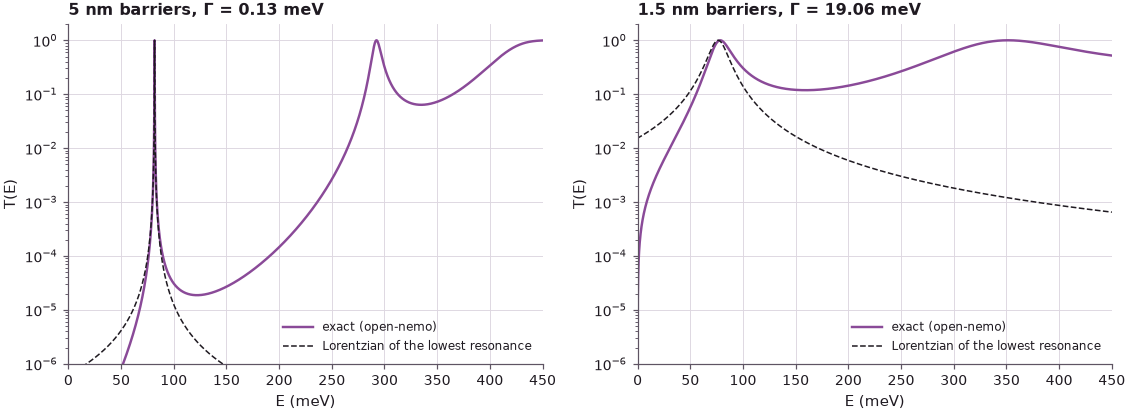
Figure computed by the notebook with open-nemo

For the 5 nm barriers ($\Gamma = 0.129$ meV, 0.005 $k_BT$) the two currents agree to within 0.1 % at 4 K; at 300 K the Landauer current is 4 % and 10 % larger, because thermally excited electrons also pass through the broad upper resonance and the background, which the single level of the rate equation does not have. As the barriers thin, the resonance broadens to 19 meV (1.5 nm) and 32 meV (1 nm), comparable to $k_BT$ and to the window, the upper resonance merges into the continuum above the barriers, and the Lorentzian no longer describes the transmission (right panel). At 4 K the sequential formula then overestimates the current by up to 27 % (1 nm: ratio 0.789), because part of the broad line lies outside the window. The coincidence of the two expressions is a property of narrow, isolated resonances. Klimeck summarizes: they part company when coherence matters, with interference between resonances and broad overlapping states.

2. Occupation: the rate equation has it, Landauer does not#

The deeper difference is the charge. The sequential picture has a well-defined occupation of the state in the centre of the well,

n = \frac{\Gamma_Lf_L + \Gamma_Rf_R}{\Gamma_L + \Gamma_R}.

Under the hood it assumes that an electron hops in, rattles around, interacts with other electrons or with phonons, comes to some sort of local equilibrium, and hops out: sequential tunneling usually implies scattering or decoherence. The Landauer formula, $I = (2e/h)\int T(f_L - f_R)\,dE$, contains no expression for the charge inside the device at all; only the reservoirs are well defined, each with its own Fermi level. For the charge one needs a quantum transport method that populates the states of the device out of equilibrium, such as NEGF.

In NEGF the states injected from the left contact have the spectral function $A_L(z, E)$ and those from the right $A_R(z, E)$; the density is

n(z) = \int\frac{dE}{2\pi}\Bigl[A_L(z, E)f_L(E) + A_R(z, E)f_R(E)\Bigr].

Transport.solve returns both spectral functions. At large bias ($f_L = 1$, $f_R = 0$ at the resonance) the well holds the left-injected part only. Integrating $A_L$ and $A_R$ over the well and over $\pm 10\,\Gamma$ around the resonance gives the left- and right-connected parts of the state, $N_L$ and $N_R$; their ratio $N_L/(N_L + N_R)$ is the coherent counterpart of the rate-equation occupation. The rates $\Gamma_{L,R}$ are the one-sided widths of Lecture 10.2 (the other barrier made 14 nm thick).

Code30 lines · cell 6

def one_sided_rates(b_left, b_right):
    gl = nemo.resonances(double_barrier(b_left, 14.0))["width"][0]
    gr = nemo.resonances(double_barrier(14.0, b_right))["width"][0]
    return gl, gr


profiles = {}
print(" b_L  b_R (nm)   Γ_L/(Γ_L+Γ_R) rate equation   N_L (NEGF)   N_R (NEGF)   N_L/(N_L+N_R)")
for bl, br in ((3, 5), (5, 5), (5, 3)):
    dev = double_barrier(bl, br)
    res = nemo.resonances(dev)
    e0, g = res["energy"][0], res["width"][0]
    E = e0 + g * np.linspace(-10, 10, 2001)
    data = nemo.Transport(dev.hamiltonian).solve(E).data
    well = (dev.x >= 10 + bl) & (dev.x <= 15 + bl)
    n_l = np.trapezoid(data["spectral_left"][:, well].sum(axis=1), E) / (2 * np.pi)
    n_r = np.trapezoid(data["spectral_right"][:, well].sum(axis=1), E) / (2 * np.pi)
    profiles[bl, br] = (dev.x - 10 - bl, np.trapezoid(data["spectral_left"], E, axis=0) / (2 * np.pi))
    gl, gr = one_sided_rates(bl, br)
    print(f"  {bl}    {br}               {gl / (gl + gr):.4f}                {n_l:.4f}       {n_r:.4f}"
          f"         {n_l / (n_l + n_r):.4f}")

fig, ax = plt.subplots(figsize=(7, 3.6))
for (bl, br), c in zip(profiles, style.sweep(3)):
    z, dens = profiles[bl, br]
    ax.plot(z, dens / 0.05, color=c, label=f"{bl} nm | 5 nm | {br} nm")   # per nm (grid 0.05 nm)
ax.axvspan(0, 5, color=style.CONTEXT, alpha=0.12, lw=0)
ax.set(xlabel="position from the left edge of the well (nm)", ylabel="electrons per nm",
       title="left-injected density at large bias (NEGF)", xlim=(-8, 13))
ax.legend(frameon=False, fontsize=8);

 b_L  b_R (nm)   Γ_L/(Γ_L+Γ_R) rate equation   N_L (NEGF)   N_R (NEGF)   N_L/(N_L+N_R)
  3    5               0.9479                0.8187       0.0448         0.9482
  5    5               0.5000                0.4304       0.4304         0.5000
  5    3               0.0521                0.0448       0.8187         0.0518

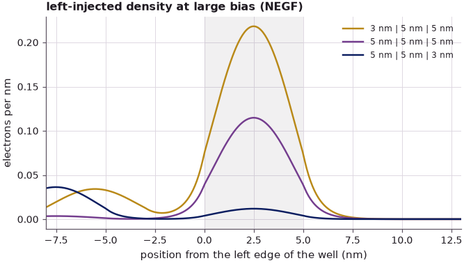
In this limit the coherent calculation and the rate equation agree on the occupation too: 0.9482 against 0.9479 for the thin source barrier, 0.5000 for the symmetric structure and 0.0518 against 0.0521 for the thick source barrier. ($N_L + N_R = 0.86$ rather than one because only part of the state lies inside the well and within $\pm 10\,\Gamma$.) The profiles show Klimeck's insight from Lecture 10.2 directly: with the thin barrier on the source side the well is full, with the thin barrier on the drain side it is nearly empty. The essential point is that this number required the spectral functions of NEGF; $T(E)$ alone could not provide it.

3. Free carriers and the potential act back on each other#

Why does the charge matter? Because the potential is not given: it follows from Poisson's equation,

\nabla^2 V(\vec r) = -\frac{\rho(\vec r)}{\epsilon},\qquad \rho(\vec r) = e\bigl[N_D^+(\vec r) - N_A^-(\vec r) + p(\vec r) - n(\vec r)\bigr],

with $\epsilon$ the permittivity, $N_D^+$ and $N_A^-$ the ionized donors and acceptors (fixed in space) and $n$, $p$ the free electrons and holes, which move, drift, diffuse and are injected. The transport calculation gives $n$ and $p$ as complicated functions of energy and voltage. If there are too few or too many carriers, the potential reacts, and the potential in turn changes the transport.

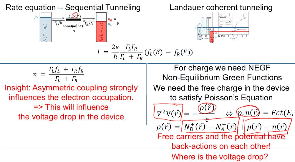
Slide 4: Poisson's equation and the back-action of the free charge — Slide 4: asymmetric coupling sets the occupation; the free charge must satisfy Poisson's equation, so free carriers and the potential act back on each other.

A one-step estimate shows how strong this is. Place a sheet of electrons with density $\sigma$ in the well, with the profile of the resonant state, and solve the one-dimensional Poisson equation for the electron potential energy $U$,

\frac{d^2U}{dz^2} = -\frac{e^2}{\epsilon_0\epsilon_r}\,n(z),\qquad \int n(z)\,dz = \sigma,

with $U = 0$ at both ends of the structure (contacts that screen perfectly), $\epsilon_0$ the vacuum permittivity and $\epsilon_r = 12.9$; the electrons' negative charge raises their potential energy. Then nemo.resonances(dev, potential=U) gives the shifted resonance. The sheet density itself depends on how many transverse states are filled (Lecture 10.7): electrons with energy $E_r$ along $z$ and any transverse energy up to $\mu_L - E_r$ occupy the resonance, so $\sigma \approx n\,g_{2D}(\mu_L - E_r)$ with $g_{2D} = m^*/\pi\hbar^2$ (both spins).

Code30 lines · cell 8

dev = double_barrier(5, 5)
res = nemo.resonances(dev)
e0, g = res["energy"][0], res["width"][0]
x = dev.x
shape = np.asarray(res["density"][0], dtype=float)
shape /= np.trapezoid(shape, x)                                     # 1/nm, integrates to one
E2_EPS0 = Q / 8.8541878128e-12 * 1e9                                # e/ε0 in V nm


def hartree_potential(sigma_cm2, eps_r=12.9):
    # U'' = -e²/(ε0 εr) n(z), U = 0 at both ends (finite differences), U in eV
    n = sigma_cm2 * 1e-14 * shape                                   # electrons per nm³
    h = x[1] - x[0]
    m = len(x) - 2
    lap = (np.diag(-2 * np.ones(m)) + np.diag(np.ones(m - 1), 1) + np.diag(np.ones(m - 1), -1)) / h**2
    u = np.zeros_like(x)
    u[1:-1] = np.linalg.solve(lap, -E2_EPS0 / eps_r * n[1:-1])
    return u


print(" σ (cm⁻²)    max U (meV)   E_r (meV)   shift (meV)   shift / Γ")
for sigma in (0, 1e9, 1e10, 1e11, 5e11):
    u = hartree_potential(sigma)
    er = nemo.resonances(dev, potential=u)["energy"][0]
    print(f" {sigma:8.0e}      {u.max() * 1e3:7.2f}      {er * 1e3:7.2f}      {(er - e0) * 1e3:6.2f}"
          f"      {(er - e0) / g:7.1f}")
g2d = 0.067 / (2 * np.pi * H2M0) * 1e14                             # m*/πħ² in cm⁻² eV⁻¹
print(f"\ng_2D = m*/πħ² = {g2d:.3e} cm⁻² eV⁻¹")
for n_occ in (0.948, 0.052):
    print(f"n = {n_occ}: σ ≈ n g_2D (20 meV) = {n_occ * g2d * 0.02:.2e} cm⁻²")

 σ (cm⁻²)    max U (meV)   E_r (meV)   shift (meV)   shift / Γ
    0e+00         0.00        81.79        0.00          0.0
    1e+09         0.11        81.90        0.11          0.8
    1e+10         1.13        82.89        1.10          8.5
    1e+11        11.33        92.75       10.96         84.8
    5e+11        56.63       136.59       54.80        423.9

g_2D = m*/πħ² = 2.799e+13 cm⁻² eV⁻¹
n = 0.948: σ ≈ n g_2D (20 meV) = 5.31e+11 cm⁻²
n = 0.052: σ ≈ n g_2D (20 meV) = 2.91e+10 cm⁻²

A sheet of only $10^{10}$ cm$^{-2}$ electrons raises the potential in the well by 1.13 meV and moves the resonance up by 1.10 meV, 8.5 widths; at $10^{11}$ cm$^{-2}$ the shift is 11.0 meV, and at $5\cdot10^{11}$ cm$^{-2}$ it is 54.8 meV, two thirds of the resonance energy itself. With $\mu_L$ 20 meV above the resonance the full level of the 3 nm | 5 nm structure holds about $5\cdot10^{11}$ cm$^{-2}$, the nearly empty level of the 5 nm | 3 nm structure 18 times less: the two structures have the same coherent current at a fixed potential, but completely different potentials, and so different currents, once the charge is included. Sequential and coherent tunneling give the same current whenever the resonance is narrow and isolated, but neither gives it at the right bias without the charge and Poisson's equation. Where the voltage drops is the subject of Lectures 10.5 and 10.6.

Summary#

Sequential tunneling (rate equation) and coherent tunneling (Landauer) give the same current, $(2e/\hbar)\,\Gamma_L\Gamma_R/(\Gamma_L + \Gamma_R)\,(f_L - f_R)$, for a narrow, isolated resonance; the agreement degrades as the resonance broadens toward $k_BT$ and the window and as other states contribute.
The rate equation defines an occupation of the well and implies decoherence. The Landauer formula defines no charge in the device; NEGF does, through the spectral functions $A_L$ and $A_R$.
At large bias the NEGF occupation of the well state, $N_L/(N_L + N_R)$, equals the rate-equation $\Gamma_L/(\Gamma_L + \Gamma_R)$: 0.948 for a thin source barrier, 0.052 for a thick one.
The free charge enters Poisson's equation: $10^{10}$ cm$^{-2}$ in the well already moves the resonance by several widths. Free carriers and the potential act back on each other.

Exercises#

Repeat the width comparison of Section 1 for asymmetric barriers (3 nm | 5 nm). Is the agreement between the two currents better or worse than for the symmetric structure of the same total width?
Compute the density $n(z)$ of Section 2 at a finite temperature and bias, with $f_L$ and $f_R$ evaluated over a wide energy grid, for $\mu_L = E_r + 20$ meV and $\mu_R = \mu_L - 0.2$ eV. How much charge sits in the well, and how much in the emitter contact region?
Build a triple-barrier structure (two 5 nm wells separated by a 2 nm barrier). Compare its exact $T(E)$ with the sum of two Lorentzians at the two resonances. Where does interference make the difference?