

Lecture 23.2
Theory of stress and strain — deformation: strain
In the lecture
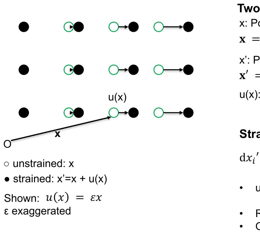
- Two vectors describe a deformed crystal: the reference position \(\mathbf{x}\) of an atom and its displacement \(\mathbf{u}(\mathbf{x})\); strain is the change of distances, so only the gradient \(\partial u_i/\partial x_j\) matters.
- Rigid translations and rigid rotations move atoms but produce no strain.
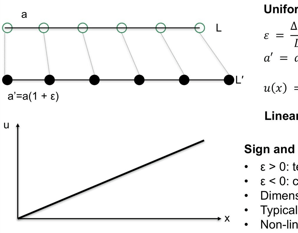
- In one dimension a uniform stretch \(a' = a(1+\varepsilon)\) means a linear displacement \(u = \varepsilon x\) and a constant strain \(\varepsilon = \mathrm{d}u/\mathrm{d}x\); a nonlinear \(u(x)\) gives a local strain.
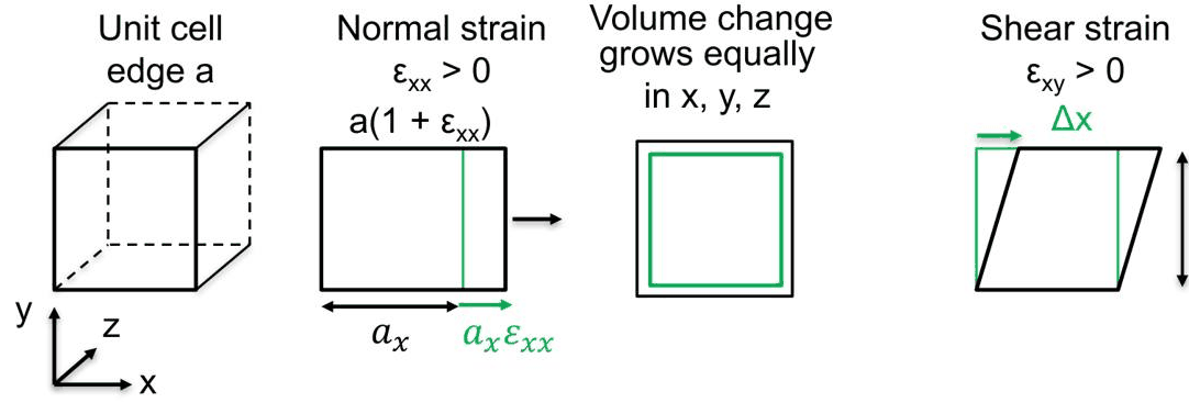
- In three dimensions the strain tensor \(\varepsilon_{ij} = \tfrac12(\partial u_i/\partial x_j + \partial u_j/\partial x_i)\): diagonal entries stretch the cell, its trace is the volume change, off-diagonal entries are shear.
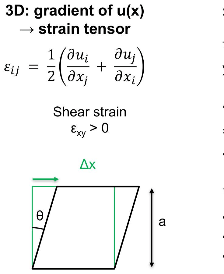
- Simple shear and the origin of the factor 2: the right angle of the cell closes by \(\theta \approx 2\varepsilon_{xy}\).
In this notebook
You compute displacement gradients of translated, rotated and stretched grids of atoms and see which of them carry strain; build a one-dimensional chain with a strained inclusion and read the local strain off its atoms; deform a GaAs unit cell with mechanics.strain_structure, recover the strain tensor from its bonds with mechanics.atomic_strain, and compare the trace with the exact volume change; and check the shear angle \(\theta \approx 2\varepsilon_{xy}\), including the internal relaxation of the atoms that continuum theory does not see.
Run it on your own machine
The notebook needs open-nemo (Python ≥ 3.10 and a C++20 compiler; BLAS/LAPACK).
git clone https://github.com/denphi/open-nemo.git && cd open-nemo
python3 -m venv .venv && source .venv/bin/activate
pip install -e ".[notebooks]"
jupyter lab From_Atoms_to_Devices/09_stress_and_strain/23_2_deformation_strain.ipynbCode
import numpy as np
import matplotlib.pyplot as plt
import opennemo as nemo
from opennemo.visualization import style
from opennemo.models import mechanics as M
from opennemo.solvers import elasticity as E
from opennemo.structures.structure import Structure

style.use(notebook=True)
1. Where atoms sit and how far they move#
Strain is geometry. Take a crystal in its unstrained reference state and label every atom by its position there, \(\mathbf{x} = (x, y, z) \equiv (x_1, x_2, x_3)\). (The points could equally be the nodes of a finite-element mesh; the definitions are the same.) After the crystal is deformed the atom that started at \(\mathbf{x}\) sits at
where \(\mathbf{u}(\mathbf{x})\) is the displacement: how far that particular atom has moved. Strain is the change of distances between atoms. Two neighbouring atoms separated by \(\mathrm{d}\mathbf{x}\) before the deformation are separated afterwards by
Only the gradient \(\partial u_i/\partial x_j\) enters. A constant displacement moves every atom by the same amount, a rigid translation: its derivative is zero and there is no strain. A rigid rotation changes the directions of the bonds but not their lengths, and is not strain either.
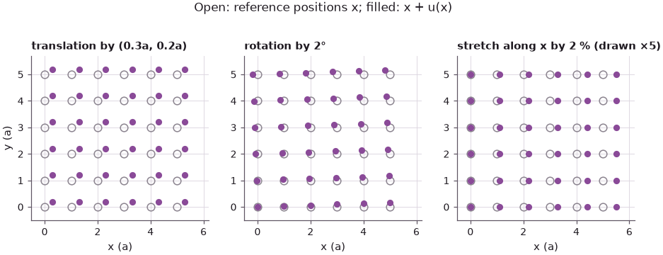
The three cases of the slide can be checked on a small grid of atoms. The cell below applies a rigid translation, a rigid rotation by 2° and a uniform stretch of 2 % along \(x\), and computes the gradient \(\partial u_i/\partial x_j\) numerically from the displaced positions.
Code
a = 1.0                                         # grid spacing (arbitrary length unit)
X, Y = np.meshgrid(np.arange(6) * a, np.arange(6) * a, indexing="xy")
th = np.radians(2.0)
fields = {                                      # displacement (u_x, u_y) of the atom at (X, Y)
    "translation by (0.3a, 0.2a)": (0.3 * a + 0 * X, 0.2 * a + 0 * Y),
    "rotation by 2°": (X * np.cos(th) - Y * np.sin(th) - X, X * np.sin(th) + Y * np.cos(th) - Y),
    "stretch along x by 2 %": (0.02 * X, 0 * Y),
}

def gradient(ux, uy):
    # du_i/dx_j at the central atom, from finite differences on the grid (rows y, columns x)
    g = [np.gradient(u, a) for u in (ux, uy)]          # np.gradient returns (d/dy, d/dx)
    return np.array([[gi[1][2, 2], gi[0][2, 2]] for gi in g])

for name, (ux, uy) in fields.items():
    du = gradient(ux, uy)
    eps = 0.5 * (du + du.T)                       # symmetric part: the strain tensor
    print(f"{name:28s} du/dx = {np.round(du, 4).tolist()}   strain = {np.round(eps, 4).tolist()}")
translation by (0.3a, 0.2a)  du/dx = [[0.0, 0.0], [0.0, 0.0]]   strain = [[0.0, 0.0], [0.0, 0.0]]
rotation by 2°               du/dx = [[-0.0006, -0.0349], [0.0349, -0.0006]]   strain = [[-0.0006, -0.0], [-0.0, -0.0006]]
stretch along x by 2 %       du/dx = [[0.02, 0.0], [0.0, 0.0]]   strain = [[0.02, 0.0], [0.0, 0.0]]
The translation has a zero gradient. The 2° rotation has a large gradient, \(\pm0.0349\) in the off-diagonal
entries, but it is antisymmetric, \(\partial u_x/\partial y = -\partial u_y/\partial x\), and drops out of the
symmetric combination that defines the strain (Section 3). What remains on the diagonal, \(-0.0006\), is
\(\cos\theta - 1 \approx -\theta^2/2\): linear theory is exact only to first order in the gradient, and a
finite rotation leaves a second-order residue. Exact measures of strain built from the deformation
gradient \(F = 1 + \partial\mathbf{u}/\partial\mathbf{x}\) remove the rotation completely.
elasticity.finite_strain provides them; the Green–Lagrange strain \(\tfrac12(F^\mathrm{T}F - 1)\) of the
rotation is zero to machine precision:
Code
R = np.array([[np.cos(th), -np.sin(th), 0], [np.sin(th), np.cos(th), 0], [0, 0, 1]])   # F of the rotation
for measure in ("infinitesimal", "green_lagrange", "biot"):
    e = E.finite_strain(R, measure)
    print(f"{measure:15s} ε_xx = {e[0, 0]:+.2e}   ε_xy = {e[0, 1]:+.2e}")
infinitesimal   ε_xx = -6.09e-04   ε_xy = +0.00e+00
green_lagrange  ε_xx = +0.00e+00   ε_xy = -1.08e-18
biot            ε_xx = +0.00e+00   ε_xy = +0.00e+00
Code
fig, axs = plt.subplots(1, 3, figsize=(10, 3.6))
for ax, (name, (ux, uy)) in zip(axs, fields.items()):
    scale = 5 if name.startswith("stretch") else 1               # exaggerate the 2 % stretch
    ax.plot(X, Y, "o", mfc="none", color=style.CONTEXT, ms=7)
    ax.plot(X + scale * ux, Y + scale * uy, "o", color=style.OPEN_NEMO, ms=5)
    ax.set_title(name + (" (drawn ×5)" if scale > 1 else ""), fontsize=10)
    ax.set_xlabel("x (a)")
    ax.set_xlim(-0.5, 6.2)
    ax.set_ylim(-0.5, 5.7)
    ax.set_aspect("equal")
axs[0].set_ylabel("y (a)")
fig.suptitle("Open: reference positions x; filled: x + u(x)", fontsize=11)
plt.show()
2. Strain in one dimension#
Stretch a chain of atoms of spacing \(a\) and length \(L\) uniformly to the length \(L' = L + \Delta L\). Every spacing grows in the same proportion, \(a' = a(1+\varepsilon)\), with the strain
The atom that started at \(x\) moves by \(u(x) = \varepsilon x\), a linear displacement, and \(\varepsilon = \mathrm{d}u/\mathrm{d}x\) is the same everywhere. A positive strain is tensile (stretched), a negative strain compressive (squeezed). Strain has no unit; it is quoted in per cent. Typical epitaxial strains are 0.1 % to a few per cent, and anything beyond that counts as very large. If \(u(x)\) is not linear, \(\varepsilon(x) = \mathrm{d}u/\mathrm{d}x\) varies from place to place. That is the situation of a quantum dot, where the strain changes from atom to atom.
A one-dimensional caricature of a quantum dot shows a nonlinear \(u(x)\). A chain of 41 GaAs-like atoms is clamped at both ends; the 10 bonds in the middle belong to an "InAs" inclusion whose natural length is 7.2 % longer. Treat each bond as a spring of natural length \(\ell_k\) and stiffness \(k_k\) (taken proportional to \(C_{11}/\ell_k\) of the material, with the measured \(C_{11}\) of 122.1 GPa and 83.3 GPa). With both ends fixed all springs carry the same force \(f\), and the total length \(L = \sum_k(\ell_k + f/k_k)\) fixes it: \(f = (L - \sum_k \ell_k)/\sum_k k_k^{-1}\).
Code
a_g, a_i = 0.56533, 0.60584                     # nm; one spring per lattice constant
c11_g, c11_i = 122.1, 83.3                                       # GPa
N = 40                                                           # bonds; 41 atoms
inclusion = (np.arange(N) >= 15) & (np.arange(N) < 25)
ell = np.where(inclusion, a_i, a_g)                              # natural bond lengths
k = np.where(inclusion, c11_i, c11_g) / ell                      # bond stiffness (arbitrary units)
L = N * a_g                                                      # ends clamped to the GaAs chain
f = (L - ell.sum()) / (1 / k).sum()
xp = np.concatenate([[0.0], np.cumsum(ell + f / k)])             # strained positions x'
x = np.arange(N + 1) * a_g                                       # reference: the unstrained GaAs chain
u = xp - x
eps_ref = np.diff(u) / a_g                                       # du/dx against the GaAs reference
eps_own = np.diff(xp) / ell - 1                                  # each bond against its own natural length
print(f"strain in the inclusion (own reference): {100 * eps_own[inclusion][0]:+.2f} %")
print(f"strain in the GaAs arms:                {100 * eps_own[~inclusion][0]:+.2f} %")
print(f"du/dx in the inclusion, against GaAs:   {100 * eps_ref[inclusion][0]:+.2f} %")
print(f"displacement at the two ends of the inclusion: {10 * u[15]:+.3f} Å and {10 * u[25]:+.3f} Å")
strain in the inclusion (own reference): -2.30 %
strain in the GaAs arms:                -1.57 %
du/dx in the inclusion, against GaAs:   +4.70 %
displacement at the two ends of the inclusion: -1.329 Å and +1.329 Å
Code
fig, (ax1, ax2) = plt.subplots(2, 1, figsize=(7.5, 5.2), sharex=True)
ax1.plot(x, 10 * u, "o-", ms=3, color=style.OPEN_NEMO)
ax1.set_ylabel("displacement u (Å)")
ax1.set_title("A clamped chain with a 10-bond 'InAs' inclusion")
xm = 0.5 * (x[1:] + x[:-1])
ax2.step(xm, 100 * eps_own, where="mid", color=style.OPEN_NEMO, label="against its own bond length")
ax2.step(xm, 100 * eps_ref, where="mid", color=style.CONTEXT, ls="--", label="du/dx against GaAs")
ax2.axhline(0, color="k", lw=0.6)
ax2.set_xlabel("reference position x (nm)")
ax2.set_ylabel("strain (%)")
ax2.legend(fontsize=8)
for ax in (ax1, ax2):
    ax.axvspan(x[15], x[25], color="0.9", zorder=0)
plt.show()
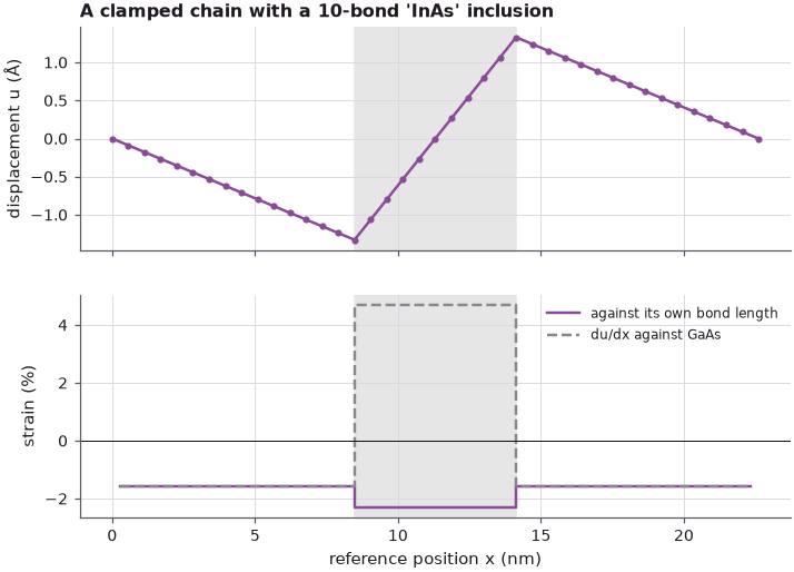
The displacement is piecewise linear and its slope, the strain, piecewise constant. The inclusion needs more room than the clamped chain offers, so the whole chain is under compression: every spring carries the same force, and the softer inclusion takes the larger share, \(-2.30\,\%\), against \(-1.57\,\%\) in the GaAs arms. The displacement falls along the left arm, reaching \(-1.329\) Å at the inclusion, rises across the inclusion to \(+1.329\) Å and falls back to zero along the right arm. The plot also shows that the number depends on the reference. Measured against the GaAs chain, \(\mathrm{d}u/\mathrm{d}x\) in the inclusion is \(+4.70\,\%\) (its bonds are still longer than GaAs bonds); measured against the inclusion's own lattice constant, which is what decides its forces and its band edges, it is compressive. Lecture 23.5 returns to this distinction for a thin InAs layer on GaAs.
3. The strain tensor in three dimensions#
In three dimensions the gradient \(\partial u_i/\partial x_j\) is a 3 × 3 matrix. Its symmetric part is the strain tensor
the antisymmetric part is the local rotation, which, as in Section 1, is not strain. A diagonal entry \(\varepsilon_{ii}\) is the relative stretch of the cell along \(i\): the edge \(a\) becomes \(a(1+\varepsilon_{xx})\). The sum of the diagonal entries is the relative change of volume,
so a uniform expansion by \(\varepsilon\) along all three axes changes the volume by \(3\varepsilon\). The off-diagonal entries are shear: they tilt the cell edges and change angles, not the volume.
The cell below takes the 8-atom conventional cell of GaAs, applies three homogeneous strains with
mechanics.strain_structure (letting the atoms relax inside the strained cell with the Keating force
field), and then reads the strain tensor back off the deformed bonds of every atom with
mechanics.atomic_strain, which is how strain is extracted from atomistic simulations (and from
NEMO 3-D). The exact volume change is \(\det(1+\boldsymbol{\varepsilon}) - 1\).
Code
G = nemo.structures.materials.load("klimeck2002_sp3d5s")["GaAs"]
lat = nemo.structures.lattice.from_material(G)
cell = Structure(lat.conventional_basis, lat.conventional_species, lat.conventional,
                 lat.conventional_sublattice, lat)
vol = lambda s: abs(np.linalg.det(s.periods))
cases = {
    "normal  ε_xx = 1 %": np.diag([0.01, 0, 0]),
    "uniform ε = 1 %": 0.01 * np.eye(3),
    "shear   ε_xy = 0.5 %": np.array([[0, 0.005, 0], [0.005, 0, 0], [0, 0, 0]]),
}
for name, eps in cases.items():
    d = M.strain_structure(cell, eps, model=M.Keating)
    e = M.atomic_strain(cell, d)["strain"].mean(axis=0)             # average over the 8 atoms
    voigt = 100 * E.strain_to_voigt(e)
    print(f"{name:22s} recovered (xx, yy, zz, 2yz, 2xz, 2xy) % = {np.round(voigt, 3)}")
    print(f"{'':22s} Tr ε = {100 * np.trace(e):.4f} %,  exact ΔV/V = {100 * (vol(d) / vol(cell) - 1):.4f} %")
normal  ε_xx = 1 %     recovered (xx, yy, zz, 2yz, 2xz, 2xy) % = [ 1. -0. -0.  0.  0.  0.]
                       Tr ε = 1.0000 %,  exact ΔV/V = 1.0000 %
uniform ε = 1 %        recovered (xx, yy, zz, 2yz, 2xz, 2xy) % = [ 1.  1.  1. -0.  0.  0.]
                       Tr ε = 3.0000 %,  exact ΔV/V = 3.0301 %
shear   ε_xy = 0.5 %   recovered (xx, yy, zz, 2yz, 2xz, 2xy) % = [ 0. -0. -0. -0. -0.  1.]
                       Tr ε = -0.0000 %,  exact ΔV/V = -0.0025 %
The bonds return the applied strain exactly. For the uniform expansion the trace, 3 %, differs from the exact volume change, 3.0301 % \(= 1.01^3 - 1\), by second-order terms; for the shear the volume changes only in second order too, by \(-\varepsilon_{xy}^2 = -0.0025\,\%\). At the strains of epitaxy, a few per cent at most, the linear expressions are accurate to a few hundredths of a per cent, which is why the whole of continuum elasticity can be built on them.
The rotation test of Section 1 can be repeated on real bonds. atomic_strain fits a local deformation
gradient \(F\) to every atom's four bonds; its default (Biot) definition removes the rotation by the polar
decomposition \(F = RU\), while the cube_edges definition (the one NEMO 3-D prints) keeps it.
Code
rot = Structure(cell.positions @ R.T, cell.species, cell.periods @ R.T, cell.sublattice, lat)
for definition in ("biot", "cube_edges"):
    e = M.atomic_strain(cell, rot, definition=definition)["strain"][0]
    print(f"{definition:10s} strain of atom 0 after a 2° rotation:\n{np.round(e, 5)}")
biot       strain of atom 0 after a 2° rotation:
[[-0.  0.  0.]
 [ 0. -0. -0.]
 [ 0. -0.  0.]]
cube_edges strain of atom 0 after a 2° rotation:
[[-0.00061 -0.0349  -0.     ]
 [ 0.0349  -0.00061  0.     ]
 [ 0.      -0.       0.     ]]
With the rotation removed the strain of a rigidly rotated crystal is zero. The cube_edges output
contains the rotation (\(\pm0.0349 = \pm\sin 2°\) off the diagonal) and its second-order residue on the
diagonal: when reading strain files produced by other codes it matters which definition they use.
4. Shear strain and the factor 2#
Why the \(\tfrac12\) in the definition, and what does an off-diagonal entry look like? Take simple shear: the bottom edge of a cell of height \(a\) stays fixed and the top edge slides by \(\Delta x\), so that
The side edges tilt by the angle \(\theta\) with \(\tan\theta = \Delta x/a = 2\varepsilon_{xy}\), and for small strain, \(|\varepsilon| \ll 1\), \(\theta \approx 2\varepsilon_{xy}\) in radians. The right angle of the cell closes by \(\theta\); edge lengths and volume are unchanged to first order. Engineers often quote the engineering shear strain \(\gamma_{xy} = 2\varepsilon_{xy}\), the angle itself; the Voigt vectors printed above use it (their last entry is \(2\varepsilon_{xy}\)).
Code
print(" ε_xy (%)   θ = atan(2ε_xy) (°)   2ε_xy (°)   rel. difference")
for exy in (0.001, 0.005, 0.01, 0.05):
    t_exact, t_lin = np.degrees(np.arctan(2 * exy)), np.degrees(2 * exy)
    print(f"{100 * exy:8.1f}   {t_exact:16.4f}   {t_lin:11.4f}   {(t_lin - t_exact) / t_exact:12.1e}")
d = M.strain_structure(cell, cases["shear   ε_xy = 0.5 %"], model=M.Keating)
p1, p2 = d.periods[0], d.periods[1]
angle = np.degrees(np.arccos(p1 @ p2 / np.linalg.norm(p1) / np.linalg.norm(p2)))
print(f"angle between the a1 and a2 edges of the sheared GaAs cell: {angle:.4f}° (90° − {90 - angle:.4f}°)")
 ε_xy (%)   θ = atan(2ε_xy) (°)   2ε_xy (°)   rel. difference
     0.1             0.1146        0.1146        1.3e-06
     0.5             0.5729        0.5730        3.3e-05
     1.0             1.1458        1.1459        1.3e-04
     5.0             5.7106        5.7296        3.3e-03
angle between the a1 and a2 edges of the sheared GaAs cell: 89.4270° (90° − 0.5730°)
At the slide's \(\varepsilon_{xy} = 0.5\,\%\) the angle is 0.5729° (the linear estimate 0.5730° is off by
3.3e-5 of itself), and the two cube edges of the sheared GaAs cell meet at 89.4270°. Note that
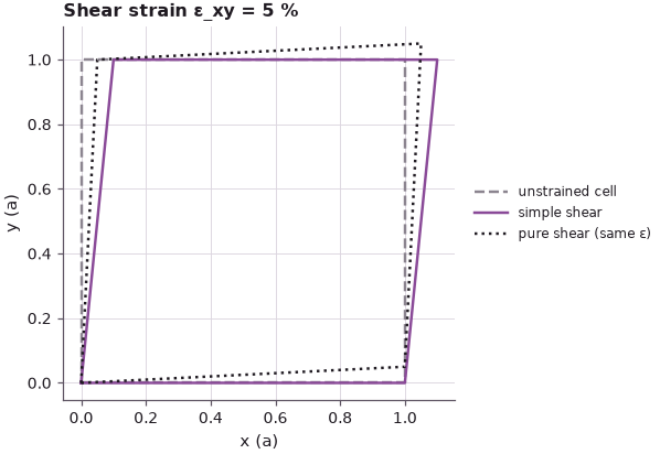
strain_structure applies the symmetric tensor, pure shear, in which both edges tilt towards each other
by \(\varepsilon_{xy}\); simple shear tilts one edge by \(2\varepsilon_{xy}\). The two have the same strain
tensor and differ by a rigid rotation through \(\varepsilon_{xy}\), the antisymmetric part of the gradient:
Code
exy = 0.05                                                          # exaggerated, to be visible
square = np.array([[0, 0], [1, 0], [1, 1], [0, 1], [0, 0]], float)
simple = square @ np.array([[1, 2 * exy], [0, 1]]).T                # u_x = 2 ε_xy y
pure = square @ np.array([[1, exy], [exy, 1]]).T                    # symmetric: both edges tilt
fig, ax = plt.subplots(figsize=(6.4, 4.0))
ax.plot(*square.T, color=style.CONTEXT, ls="--", label="unstrained cell")
ax.plot(*simple.T, **style.series(), label="simple shear")
ax.plot(*pure.T, **style.series("reference"), label="pure shear (same ε)")
ax.set_aspect("equal")
ax.set_xlabel("x (a)")
ax.set_ylabel("y (a)")
ax.set_title(f"Shear strain ε_xy = {100 * exy:.0f} %")
ax.legend(fontsize=8, loc="center left", bbox_to_anchor=(1.02, 0.5))
plt.show()
for nm, F2 in (("simple", np.array([[1, 2 * exy], [0, 1]])), ("pure", np.array([[1, exy], [exy, 1]]))):
    e = 0.5 * (F2 + F2.T) - np.eye(2)
    print(f"{nm:6s} shear: ε = {e.round(3).tolist()}, area change = {np.linalg.det(F2) - 1:+.4f}")
simple shear: ε = [[0.0, 0.05], [0.05, 0.0]], area change = +0.0000
pure   shear: ε = [[0.0, 0.05], [0.05, 0.0]], area change = -0.0025
Both shapes have \(\varepsilon_{xy} = 5\,\%\); the area of simple shear is exactly unchanged, that of pure shear changes by \(-\varepsilon_{xy}^2 = -0.25\,\%\), second order again.
One thing the continuum picture leaves out appears as soon as the cell holds more than one atom. In
zincblende the two atoms of the primitive cell do not simply follow the homogeneous shear: the Ga
sublattice shifts against the As sublattice along \(z\), which trades bond-length changes for bond-angle
changes (Kleinman's internal strain). strain_structure relaxes the atoms with the force field, so the
shift can be read off by comparing with the homogeneously strained cell:
Code
eps = cases["shear   ε_xy = 0.5 %"]
homog = M.strain_structure(cell, eps)                               # no model: every atom follows ε
relax = M.strain_structure(cell, eps, model=M.Keating)
shift = relax.positions - homog.positions
ga = np.array(cell.species) == "Ga"
uz = np.abs(shift[ga, 2]).max()
print(f"internal shift of the Ga atoms along z: {1000 * uz:.3f} pm")
print(f"Kleinman parameter ζ = u_z / (a ε_xy / 2) = {uz / (G.lattice_constant * eps[0, 1] / 2):.3f};  "
      f"Keating (α − β)/(α + β) = {(41.19 - 8.95) / (41.19 + 8.95):.3f}")
internal shift of the Ga atoms along z: 0.909 pm
Kleinman parameter ζ = u_z / (a ε_xy / 2) = 0.643;  Keating (α − β)/(α + β) = 0.643
The Ga sublattice moves by 0.909 pm, a Kleinman parameter \(\zeta = 0.643\), exactly the Keating value \((\alpha-\beta)/(\alpha+\beta)\) for the bond-stretching and bond-bending constants of GaAs. The strain tensor of the cell is unchanged by this shift, but the bond lengths and angles are not, and the electrons see bonds. Lecture 23.7 turns strain into band-edge shifts; atomistic tight binding needs these relaxed positions.
Summary#
- Strain describes how far atoms move relative to each other: \(\mathbf{x}' = \mathbf{x} + \mathbf{u}(\mathbf{x})\), and only the gradient \(\partial u_i/\partial x_j\) matters. Rigid translations and rotations carry no strain.
- In one dimension \(\varepsilon = \Delta L/L = \mathrm{d}u/\mathrm{d}x\); positive is tensile, negative compressive; typical epitaxial values are 0.1 % to a few per cent. In a clamped chain with a 7.2 % longer inclusion, \(u(x)\) is piecewise linear: the inclusion is compressed by 2.30 % (against its own lattice constant) and the GaAs arms by 1.57 %.
- The strain tensor is the symmetric part of the gradient; its trace is the volume change (3 % for a uniform 1 % expansion, exactly 3.0301 %), and shear changes angles, not volumes.
- In simple shear the right angle closes by \(\theta \approx 2\varepsilon_{xy}\): 0.573° at \(\varepsilon_{xy} = 0.5\,\%\). Pure and simple shear share the strain tensor and differ by a rotation.
- Atomistic strain is read off the bonds (
atomic_strain); inside a zincblende cell the sublattices relax against each other under shear (\(\zeta = 0.643\) for Keating GaAs), which the continuum strain tensor does not show.
Exercises#
- Replace the 2° rotation in Section 1 by 20°. How large is the second-order residue
\(\cos\theta - 1\) of the linear strain now, and what does
finite_strain(R, "biot")give? - Make the inclusion of Section 2 twice as long (20 bonds) and then half as long. How do the strains inside and outside change? What happens when the chain ends are free instead of clamped?
- Apply \(\varepsilon_{xy} = \varepsilon_{yz} = \varepsilon_{xz} = 0.5\,\%\) (a strain along [111]) with
strain_structureandmodel=M.Keating. Do the atoms still shift against each other? Compare with the biaxial strainnp.diag([-0.01, -0.01, 0.0093]). - Compute the Kleinman parameter of InAs with
M.kleinman_parameterand compare with GaAs.
Further reading#
- Strain along different directions
- Benchmark: the strain Hamiltonian of NEMO5
- InAs/GaAs dot strain against NEMO 3-D's published profiles
- L. Kleinman, "Deformation potentials in silicon. I. Uniaxial strain", Phys. Rev. 128, 2614 (1962).
- P. N. Keating, Phys. Rev. 145, 637 (1966).
- L. D. Landau and E. M. Lifshitz, Theory of Elasticity, 3rd ed., Pergamon (1986), §1.