Lecture 21.3

NEMO 3-D — atomistic basis: nearest-neighbour sp3d5s* tight binding

Lecture page Video Slides

In the lecture

The wavefunction is expanded in s, p, d and s* orbitals on every atom: 10 orbitals, 20 with spin.
The Hamiltonian has one on-site block per atom and one coupling block per neighbour (four in zincblende); for 52 million atoms it has order $10^9$.
Slater–Koster two-centre integrals depend on the bond's direction cosines and length; strain enters through both.
The "right" basis is critical: the sp3s* silicon of Vogl et al. has wrong conduction-band masses ("pancakes" instead of cigars), which motivated genetic-algorithm fits of new parameters (Klimeck, Boykin, Bowen) to room-temperature gaps and masses.
Holes are strongly anisotropic and non-parabolic: in GaAs the light-hole band is non-parabolic and the heavy-hole band becomes electron-like away from Γ.

In this notebook

Count the blocks and non-zeros of an sp3d5s* Hamiltonian, and compare the cost with sp3s*.
Check the Slater–Koster rule $E_{s,z} = n\,V_{sp\sigma}$ and its strain scaling $(d/d')^\eta$ on a single Ga–As bond built with open-nemo.
Compare sp3s* and sp3d5s* band structures of GaAs and InAs.
Measure the silicon conduction-band valley and masses of Vogl's sp3s* and of Boykin's sp3d5s*, and the hole anisotropy of silicon.
Reproduce the constant-$k_z$ cuts of the GaAs light- and heavy-hole bands.

Run the notebookEvery number and figure on this page comes from it. Change it, rerun it, take it further.

Download .ipynb View on GitHub

Run it on your own machine

The notebook needs open-nemo (Python ≥ 3.10 and a C++20 compiler; BLAS/LAPACK).

git clone https://github.com/denphi/open-nemo.git && cd open-nemo
python3 -m venv .venv && source .venv/bin/activate
pip install -e ".[notebooks]"
jupyter lab From_Atoms_to_Devices/07_quantum_dots_and_nemo3d/21_3_sp3d5s_tight_binding.ipynb

Code27 lines · cell 1

import time
import numpy as np
import matplotlib.pyplot as plt
import opennemo as nemo
from opennemo.visualization import style
from opennemo.structures.structure import Structure, bulk, supercell
from opennemo.core import units

style.use(notebook=True)
H2M = units.HBAR2_2M0                     # hbar^2 / (2 m0) = 0.0381 eV nm^2
load = nemo.structures.materials.load
SPDS, SPS = load("klimeck2002_sp3d5s"), load("klimeck2002_sp3s")


def bulk_h(mat, spin=True):
    # tight-binding Hamiltonian of the two-atom primitive cell; h.dense(k) gives H(k)
    return nemo.models.tb.SlaterKoster(mat, spin=spin).build(bulk(nemo.structures.lattice.from_material(mat)))


def bands(h, ks):
    return np.array([np.linalg.eigvalsh(h.dense(k)) for k in ks])


def mass(f, k0, u, dk=0.02):
    # m*/m0 from a 5-point second derivative of the energy function f(k) along unit vector u (dk in 1/nm)
    e = [f(k0 + s * dk * u) for s in (-2, -1, 0, 1, 2)]
    return 2 * H2M / ((-e[0] + 16 * e[1] - 30 * e[2] + 16 * e[3] - e[4]) / (12 * dk**2))

1. The tight-binding Hamiltonian#

The electron wavefunction is written as a sum over atoms $R$ and orbitals $\alpha$ on each atom, $\psi = \sum_{R}\sum_{\alpha} C_{R\alpha}\,\phi_{R\alpha}$, with the basis s, p$_x$, p$_y$, p$_z$, five d orbitals and an excited s* orbital that stands in for higher states: 10 orbitals per atom, 20 with spin. The Hamiltonian in second quantization (slide 3) is

H = \sum_{R}\sum_{\alpha,\alpha'} \varepsilon_{R\alpha\alpha'}\,c^\dagger_{R\alpha}c_{R\alpha'} + \sum_{R}\sum_{R'\in\mathrm{nn}(R)}\sum_{\alpha,\alpha'} t_{R\alpha,R'\alpha'}\,c^\dagger_{R\alpha}c_{R'\alpha'} ,

where $c^\dagger$ and $c$ create and annihilate an electron in an orbital, $\varepsilon$ are the on-site energies (with spin–orbit coupling, a matrix on each atom) and $t$ the couplings to the four nearest neighbours $R'$. Each row of the matrix therefore has one diagonal block and four neighbour blocks. An atomistic basis carries the crystal's directions automatically: the structure, and hence the waves propagating in it, look different along [100], [110] and [111].

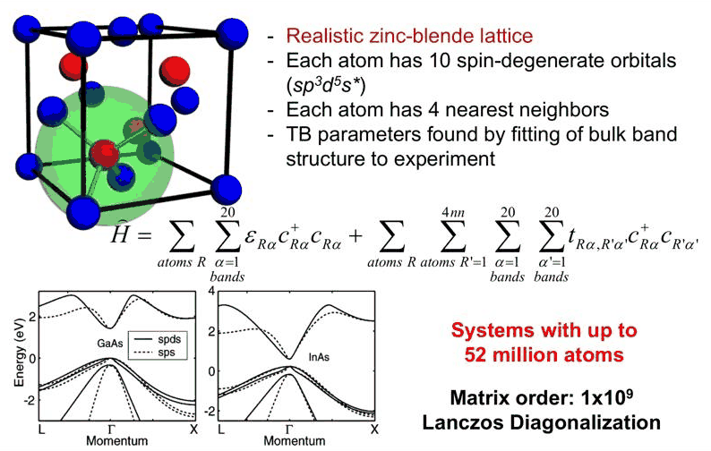
Slide 3: the nearest-neighbour sp3d5s* model

Slide 3: zincblende cell with four nearest neighbours, the Hamiltonian, and the bulk bands of GaAs and InAs in sp3d5s\ (solid) and sp3s* (dashed). Systems of up to 52 million atoms give matrices of order $10^9$.*

Code12 lines · cell 3

GAAS = SPDS["GaAs"]
lat = nemo.structures.lattice.from_material(GAAS)
cube = supercell(lat, 4)
for name, mat in (("sp3s*", SPS["GaAs"]), ("sp3d5s*", GAAS)):
    sk = nemo.models.tb.SlaterKoster(mat, spin=True)
    lat_m = nemo.structures.lattice.from_material(mat)
    H = sk.build(supercell(lat_m, 4)).at(np.zeros(3))
    rows = H.shape[0]
    nnz_row = H.nnz / rows
    print(f"{name:8s}: {rows // cube.num_atoms:2d} orbitals per atom with spin, {rows} rows for "
          f"{cube.num_atoms} atoms, {H.nnz / rows:.0f} non-zeros per row, {H.nnz:.3e} non-zeros")
print(f"52 million atoms, sp3d5s* + spin: {52e6 * 20:.2e} rows, about {52e6 * 20 * nnz_row:.1e} non-zeros")

sp3s*   : 10 orbitals per atom with spin, 5120 rows for 512 atoms, 20 non-zeros per row, 1.014e+05 non-zeros
sp3d5s* : 20 orbitals per atom with spin, 10240 rows for 512 atoms, 41 non-zeros per row, 4.237e+05 non-zeros
52 million atoms, sp3d5s* + spin: 1.04e+09 rows, about 4.3e+10 non-zeros

With spin, sp3d5s* has twice the rows of sp3s* and about twice the non-zeros per row (41 against 20), so the matrix has 4.2 times more non-zeros and a product $H\mathbf{v}$ costs about four times more. A row has far fewer entries than the $5\times20 = 100$ of five full blocks: the hopping between atoms does not flip the spin (spin–orbit coupling acts on each atom's p orbitals), which leaves at most $5\times10$, and some Slater–Koster couplings vanish for the tetrahedral bond directions. Klimeck accepts this factor because the d orbitals give better bands and, above all, the right behaviour under strain.

2. Slater–Koster couplings and strain#

The coupling between orbitals on two neighbours is built from a few two-centre integrals $V_{ll'm}$ ($m$ = σ, π, δ) and the direction cosines $(l, m, n)$ of the bond $\mathbf{d} = d\,(l\,\mathbf{e}_x + m\,\mathbf{e}_y + n\,\mathbf{e}_z)$. For example, an s orbital on the anion and a p$_z$ orbital on the cation couple by

E_{s a, z c} = n\,V_{s a,\,p c\,\sigma} .

When strain moves the atoms, the bond becomes $\mathbf{d}' = d'(l'\mathbf{e}_x + m'\mathbf{e}_y + n'\mathbf{e}_z)$: the direction cosines change, and the integral is scaled with the bond length,

E_{s a, z c} = n'\,V_{s a,\,p c\,\sigma}\left(\frac{d}{d'}\right)^{\eta},

with an exponent $\eta$ fitted for each integral (in NEMO 3-D's parameters, together with strain-dependent on-site energies; Boykin et al. 2002). The cell below builds a single Ga–As bond with open-nemo and reads the coupling of the Ga s orbital to the As p$_z$ orbital.

Code24 lines · cell 5

d0 = np.sqrt(3) / 4 * GAAS.lattice_constant
eta = GAAS.strain["exponent"]["sp_sigma"]
norb = len(GAAS.orbitals)                            # s, px, py, pz, 5 d, s*
S_GA, PZ_AS = 0, norb + GAAS.orbitals.index("pz")


def bond_block(direction, length, strain=None):
    u = np.asarray(direction, float) / np.linalg.norm(direction)
    dimer = Structure(np.array([[0.0, 0.0, 0.0], u * length]), ["Ga", "As"], np.zeros((0, 3)))
    kw = {} if strain is None else {"strain": strain}
    sk = nemo.models.tb.SlaterKoster(GAAS, spin=False, bond_tolerance=0.1, check_bonds=False, **kw)
    return sk.build(dimer).dense(np.zeros(3)).real, u[2]


V_sp, _ = bond_block([0, 0, 1], d0)
V_sp = V_sp[S_GA, PZ_AS]
print(f"bond along z:            E(s Ga, pz As) = {V_sp:.5f} eV = V_sp_sigma")
H1, n = bond_block([1, 1, 1], d0)
print(f"bond along [111]:        E = {H1[S_GA, PZ_AS]:.5f} eV,  "
      f"n V_sp_sigma = {n * V_sp:.5f} eV  (n = {n:.4f})")
for ratio in (0.97, 1.03):
    H2, n2 = bond_block([1, 1, 1.1], ratio * d0, strain="bond_length")
    print(f"bent and {100 * (ratio - 1):+.0f} % bond: E = {H2[S_GA, PZ_AS]:.5f} eV,  "
          f"n' V (d/d')^eta = {n2 * V_sp * (1 / ratio)**eta:.5f} eV  (n' = {n2:.4f}, eta = {eta:.3f})")

bond along z:            E(s Ga, pz As) = 2.96032 eV = V_sp_sigma
bond along [111]:        E = 1.70914 eV,  n V_sp_sigma = 1.70914 eV  (n = 0.5774)
bent and -3 % bond: E = 1.89583 eV,  n' V (d/d')^eta = 1.89583 eV  (n' = 0.6140, eta = 1.385)
bent and +3 % bond: E = 1.74461 eV,  n' V (d/d')^eta = 1.74461 eV  (n' = 0.6140, eta = 1.385)

The coupling follows the slide's rule exactly: the direction cosine multiplies the integral, and a 3 % compression of the bond increases it by $(1/0.97)^{1.385}$, the bond-length exponent of this integral. The Hamiltonian of a relaxed dot is built bond by bond in this way, so the relaxed positions of lecture 21.2 enter it without any strain tensor.

3. sp3s* and sp3d5s* bands#

The two NEMO 3-D parameter sets of Klimeck et al. (2002) were both fitted to the gaps and masses of GaAs and InAs; the sp3d5s* set reproduces the bands over a wider energy range, in particular the X and L valleys of the conduction band.

Code28 lines · cell 7

a_pi = lambda mat: 2 * np.pi / mat.lattice_constant
def path(mat, n=60):
    L = 0.5 * np.ones(3) * a_pi(mat)
    X = np.array([0, 0, 1.0]) * a_pi(mat)
    s1 = np.linspace(1, 0, n)[:, None] * L
    s2 = np.linspace(0, 1, n)[1:, None] * X
    ks = np.vstack([s1, s2])
    x = np.r_[-np.linalg.norm(s1, axis=1), np.linalg.norm(s2, axis=1)]
    return ks, x


fig, axs = plt.subplots(1, 2, figsize=(11, 4.2), sharey=True)
for ax, name in zip(axs, ("GaAs", "InAs")):
    for setname, P, ls, c in (("sp3d5s*", SPDS, "-", style.OPEN_NEMO), ("sp3s*", SPS, "--", style.CONTEXT)):
        ks, x = path(P[name])
        e = bands(bulk_h(P[name]), ks)
        ax.plot(x, e, ls, color=c, lw=1)
        ax.plot([], [], ls, color=c, label=setname)
        g = bands(bulk_h(P[name]), [np.zeros(3)])[0]
        xm = bands(bulk_h(P[name]), [np.array([0, 0, 1.0]) * a_pi(P[name])])[0]
        cb = g[g > 0.3].min() if name == "GaAs" else g[g > 0.45].min()
        print(f"{name} {setname:8s}: E_c(Gamma) = {cb:.3f} eV, "
              f"lowest X conduction level {xm[xm > 0.5].min():.3f} eV")
    ax.axvline(0, color="0.6", lw=0.8)
    ax.set(xlabel="k (1/nm):  L ← Γ → X", title=name, ylim=(-4, 4))
    ax.legend(frameon=False, fontsize=8)
axs[0].set_ylabel("energy (eV)")
fig.tight_layout()

GaAs sp3d5s* : E_c(Gamma) = 1.421 eV, lowest X conduction level 1.917 eV
GaAs sp3s*   : E_c(Gamma) = 1.417 eV, lowest X conduction level 1.928 eV
InAs sp3d5s* : E_c(Gamma) = 0.594 eV, lowest X conduction level 2.507 eV
InAs sp3s*   : E_c(Gamma) = 0.602 eV, lowest X conduction level 2.503 eV

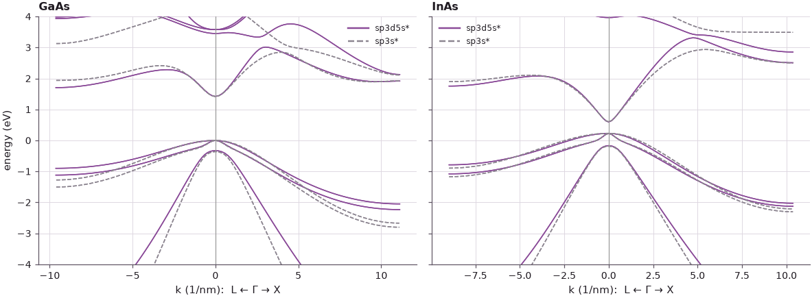
Figure computed by the notebook with open-nemo

Near the band gap the two sets agree: both were fitted to the same gaps and Γ masses. They differ away from Γ, above all in the conduction bands at X and L, and these differences matter for strain, for thin quantum wells, and for any state built from several valleys.

4. The "right" basis is critical: silicon's valleys#

Tight binding entered electrical engineering largely through Vogl, Hjalmarson and Dow's sp3s* model (1983), a set of parameters for many materials that described their energy spectra well. But in its silicon parameters, the six conduction-band valleys near X, which should be cigar-shaped ellipsoids (heavy along the valley axis, light across), come out as "pancakes": the masses are wrong. A quantization calculation with these parameters would be completely wrong even where the band edge is right.

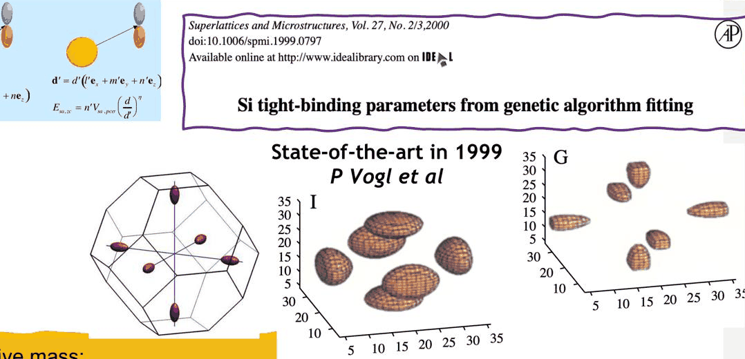
Slide 5: the silicon conduction-band constant-energy surfaces of the sp3s\ parameters of Vogl et al., pancakes rather than cigars, and the genetic-algorithm fit of new silicon parameters (Klimeck, Bowen, Boykin et al., Superlattices and Microstructures 27, 2000).*

Klimeck therefore fitted parameters to measured data with genetic algorithms, then with Tim Boykin and Chris Bowen refined the model over a series of papers: hard to publish at the time, now among the most cited parameterizations. The targets are room-temperature gaps and masses, since devices operate at room temperature, taken from experiment where possible and from DFT or k·p otherwise; the fits reach errors of a few per cent. For silicon the conduction-band minimum lies at 85 % of the way from Γ to X; the fit puts it at 81 %. Below: the valley position and the longitudinal and transverse masses of the two models.

Code23 lines · cell 9

def si_valley(P, spin=False):
    mat = P["Si"]
    h = bulk_h(mat, spin=spin)
    X = a_pi(mat)
    def ec(k):
        e = np.linalg.eigvalsh(h.dense(k))
        return e[e > 0.6].min()
    t = np.linspace(0.6, 1.0, 81)
    e = [ec(np.array([0, 0, x * X])) for x in t]
    x0 = t[int(np.argmin(e))]
    k0 = np.array([0, 0, x0 * X])
    ml = mass(ec, k0, np.array([0, 0, 1.0]), dk=0.05)
    mt = mass(ec, k0, np.array([1.0, 0, 0]), dk=0.05)
    ev = np.linalg.eigvalsh(h.dense(np.zeros(3)))
    return x0, min(e) - ev[ev < 0.3].max(), ml, mt


print(f"{'':28s} {'k_min/X':>8s} {'E_g (eV)':>9s} {'m_l':>6s} {'m_t':>6s}")
print(f"{'measured (300 K)':28s} {0.85:8.2f} {1.12:9.2f} {0.92:6.2f} {0.19:6.2f}")
for label, setname in (("Vogl et al. 1983, sp3s*", "vogl1983_sp3s"),
                       ("Boykin et al. 2004, sp3d5s*", "boykin2004_sp3d5s")):
    x0, eg, ml, mt = si_valley(load(setname))
    print(f"{label:28s} {x0:8.2f} {eg:9.3f} {ml:6.2f} {mt:6.2f}")

                              k_min/X  E_g (eV)    m_l    m_t
measured (300 K)                 0.85      1.12   0.92   0.19
Vogl et al. 1983, sp3s*          0.73     1.171   0.74   1.61
Boykin et al. 2004, sp3d5s*      0.81     1.147   0.89   0.20

Vogl's silicon has its valley minimum at 73 % of Γ–X, and a transverse mass (1.61) more than twice the longitudinal one (0.74): the pancake, where the measured valley is a cigar with $m_l/m_t \approx 5$. The sp3d5s* parameters put the minimum at 81 % of Γ–X, with $m_l = 0.89$ and $m_t = 0.20$, close to the measured cigar. With Vogl's parameters, confining electrons in a [001] silicon well would quantize them with the wrong mass in every valley.

5. Holes are very anisotropic#

The fits also target the hole masses along several directions, because holes in silicon and GaAs are strongly anisotropic, and getting this anisotropy right is critical for anything involving holes (and even for tunneling of electrons through the gap).

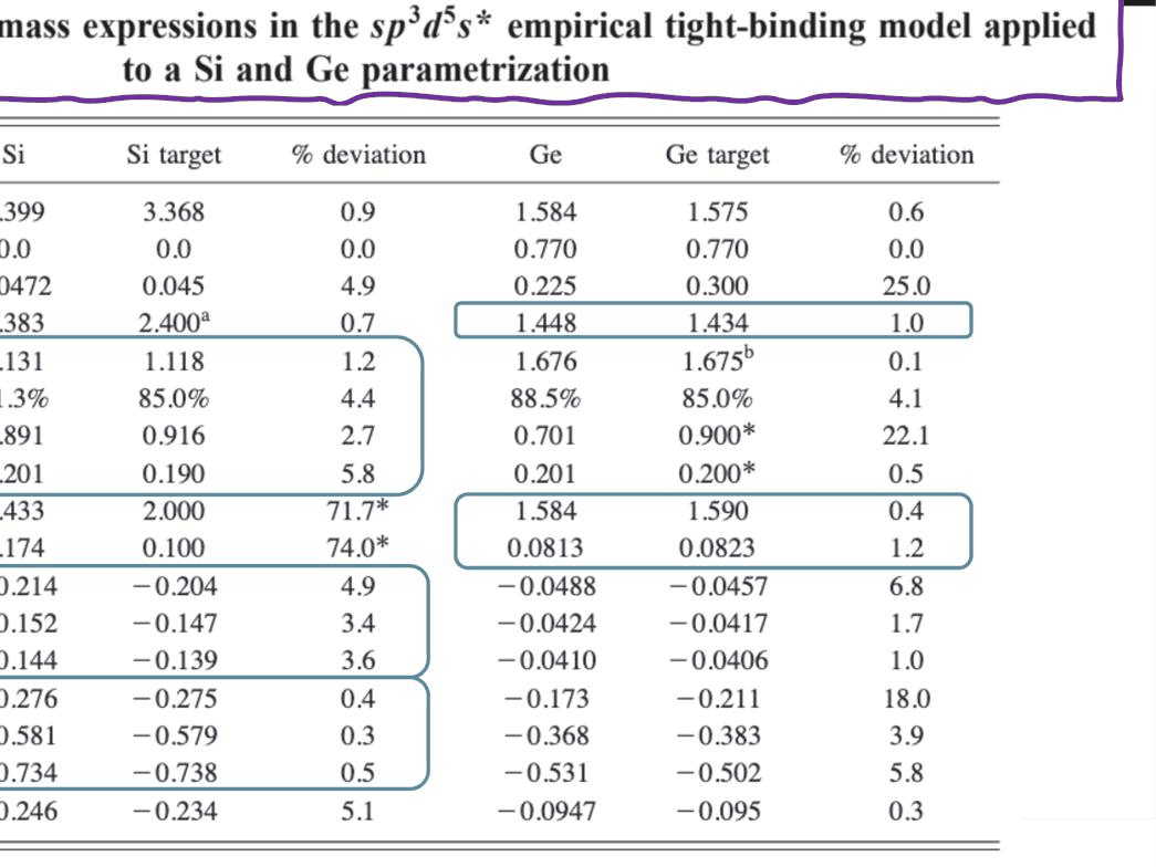
Slide 8: silicon and germanium valence-band masses

Slide 8: targets and results of the sp3d5s\ fit of Si and Ge (Boykin, Klimeck, Oyafuso, Phys. Rev. B 69, 115201 (2004)). The light-hole mass changes by 1.5× between [001] and [111], the heavy-hole mass by 2.6×.*

Code16 lines · cell 11

def pair(h, k, i):
    # energy of the i-th Kramers pair at k (with spin); pairs 2 and 3 are LH and HH at Gamma
    e = np.linalg.eigvalsh(h.dense(np.asarray(k, float)))
    return 0.5 * (e[2 * i] + e[2 * i + 1])


dirs = {"[001]": [0, 0, 1], "[011]": [0, 1, 1], "[111]": [1, 1, 1]}
slide8 = {"LH": (-0.214, -0.152, -0.144), "HH": (-0.276, -0.581, -0.734)}   # Si, sp3d5s* fit (slide 8)
h_si = bulk_h(load("boykin2004_sp3d5s")["Si"], spin=True)
print(f"{'Si':4s} " + "".join(f"{d:>9s}" for d in dirs) + "   anisotropy   (slide 8 in brackets)")
for name, i in (("LH", 2), ("HH", 3)):
    m = [mass(lambda k: pair(h_si, k, i), np.zeros(3), np.array(v, float) / np.linalg.norm(v), dk=0.01)
         for v in dirs.values()]
    r = max(np.abs(m)) / min(np.abs(m))
    print(f"{name:4s} " + "".join(f"{x:9.3f}" for x in m) + f"    {r:.2f} " + f"   ({slide8[name][0]:.3f}, "
          f"{slide8[name][1]:.3f}, {slide8[name][2]:.3f})")

Si       [001]    [011]    [111]   anisotropy   (slide 8 in brackets)
LH      -0.214   -0.152   -0.144    1.48    (-0.214, -0.152, -0.144)
HH      -0.276   -0.581   -0.734    2.66    (-0.276, -0.581, -0.734)

The heavy-hole mass of silicon grows from 0.28 along [001] to 0.73 along [111], and the light-hole mass falls from 0.21 to 0.14: the two bands are warped in opposite directions, by factors of 2.66 and 1.49, the 2.6× and 1.5× of the slide. open-nemo's masses for this parameter set are the fit's values in the table of slide 8 to all three digits. A single effective mass per band cannot describe this.

6. GaAs: non-parabolic light holes, electron-like heavy holes#

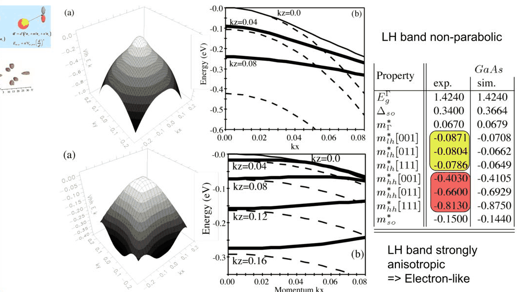
Slide 9: GaAs heavy- and light-hole dispersions — Slide 9: GaAs light-hole (top) and heavy-hole (bottom) bands in the $k_x$–$k_y$ plane, and cuts $E(k_x)$ at fixed $k_z$ (solid: tight binding, dashed: parabolic bands with the [001] masses); the table compares measured masses with the fit.

Quantizing a band in a well of width $L$ fixes $k_z$ near multiples of $\pi/L$; the in-plane dispersion of each subband then follows a cut of the bulk band at constant $k_z$. For a parabolic band each cut would be the same parabola, shifted down by $\hbar^2k_z^2/2m$. The cuts below use the NEMO 3-D sp3d5s* GaAs, with $k$ in units of $2\pi/a$ as on the slide.

Code25 lines · cell 13

h_ga = bulk_h(GAAS, spin=True)
u = 2 * np.pi / GAAS.lattice_constant
ev0 = pair(h_ga, np.zeros(3), 3)
m_lh = mass(lambda k: pair(h_ga, k, 2), np.zeros(3), np.array([0, 0, 1.0]), dk=0.01)
m_hh = mass(lambda k: pair(h_ga, k, 3), np.zeros(3), np.array([0, 0, 1.0]), dk=0.01)
print(f"GaAs [001] masses: light hole {m_lh:.4f}, heavy hole {m_hh:.4f} "
      f"(measured, slide 9: -0.0871, -0.4030)")
kx = np.linspace(0, 0.08, 41)
fig, axs = plt.subplots(1, 2, figsize=(11, 4.2))
cases = (("light hole", 2, m_lh, (0, 0.04, 0.08), (-0.6, 0.0)),
         ("heavy hole", 3, m_hh, (0, 0.04, 0.08, 0.12, 0.16), (-0.32, 0.0)))
for ax, (name, i, m, kzs, ylim) in zip(axs, cases):
    cols = style.sweep(len(kzs))
    for kz, c in zip(kzs, cols):
        e = [pair(h_ga, [x * u, 0, kz * u], i) - ev0 for x in kx]
        ax.plot(kx, e, color=c, lw=2, label=f"kz = {kz:.2f}")
        ax.plot(kx, H2M * ((kx * u)**2 + (kz * u)**2) / m, "--", color=c, lw=1)
    ax.set(xlabel="kx (2π/a)", ylabel="E − E_v (eV)",
           title=f"GaAs {name}: cuts at fixed kz (dashed: parabolic)",
           ylim=ylim)
    ax.legend(frameon=False, fontsize=8)
fig.tight_layout()
for kz in (0.08, 0.16):
    e = [pair(h_ga, [x * u, 0, kz * u], 3) - ev0 for x in (0.0, 0.08)]
    print(f"heavy hole, kz = {kz:.2f}: E(kx=0) = {e[0]:.4f} eV, E(kx=0.08) = {e[1]:.4f} eV")

GaAs [001] masses: light hole -0.0834, heavy hole -0.3768 (measured, slide 9: -0.0871, -0.4030)
heavy hole, kz = 0.08: E(kx=0) = -0.0768 eV, E(kx=0.08) = -0.0749 eV
heavy hole, kz = 0.16: E(kx=0) = -0.2766 eV, E(kx=0.08) = -0.2282 eV

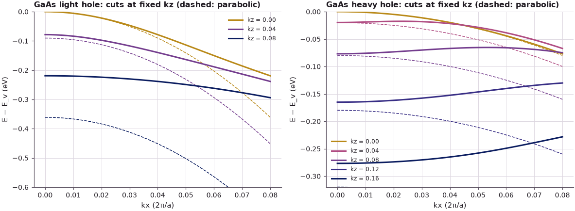
The light-hole cuts fall much less steeply than the parabola: at $k_z = 0.08$ the band lies far above the parabolic estimate, i.e. the light hole becomes heavy within a few per cent of the zone. The heavy-hole cuts at larger $k_z$ are even more striking: their energy rises with $k_x$, an electron-like dispersion: at $k_z = 0.08$ the cut is nearly flat (−0.0768 eV at $k_x = 0$, −0.0749 eV at $k_x = 0.08$), and at $k_z = 0.16$ it rises from −0.2766 eV to −0.2282 eV, the trend of slide 9. (The [001] masses of this NEMO 3-D set, −0.083 for the light and −0.377 for the heavy hole, differ from the simulated column of slide 9, which comes from another fit, but the shapes are the same.) In a quantum well of a few nanometres the excited hole subbands sample exactly these regions, so their in-plane masses can have either sign. Tight binding contains these non-parabolic, anisotropic effects in bulk, and NEMO 3-D takes the "leap of faith" of using the same bulk-fitted parameters, atom by atom, in nanostructures and under strain.

Summary#

NEMO 3-D's basis is s, p, d and s* on every atom (20 orbitals with spin); each row of the Hamiltonian has an on-site block and four neighbour blocks, and a 52-million-atom system has about $10^9$ rows.
sp3d5s* doubles the rows of sp3s* and quadruples the work per product, for better bands and correct strain behaviour.
Couplings follow Slater–Koster rules such as $E_{s,z} = n V_{sp\sigma}$, scaled by $(d/d')^\eta$ under strain — checked here on a single Ga–As bond.
Vogl's sp3s* silicon has its valley at X with $m_t > m_l$ (pancakes); the sp3d5s* fit gives 81 % of Γ–X with $m_l = 0.89$, $m_t = 0.20$.
Silicon holes are warped by factors 2.6 (heavy) and 1.5 (light) between [001] and [111]; GaAs light holes are strongly non-parabolic and heavy holes turn electron-like away from Γ.

Exercises#

Compute the GaAs heavy- and light-hole masses along [011] and [111] and compare them with the measured values in the table of slide 9.
Repeat section 4 for germanium, whose conduction-band minimum is at L: check the gap and the L masses of boykin2004_sp3d5s (if the set has Ge) or of jancu1998_sp3d5s.
Repeat the cuts of section 6 with the sp3s* GaAs (SPS["GaAs"]). Are the electron-like heavy holes still there?