Course/03 · Tunneling and band structure

ECE 606 Lecture 6.2

Electron tunneling — tunneling through a single barrier

In the lecture

the transmission \(T = |E/A|^2 = 1/|M_{11}|^2\) of a single barrier, worked out in closed form below and above the barrier top
the strong-barrier limit (\(\gamma L \gg 1\)): exponential decay with barrier width and height
the weak-barrier limit (\(\gamma L \ll 1\)): a Lorentzian in the barrier width
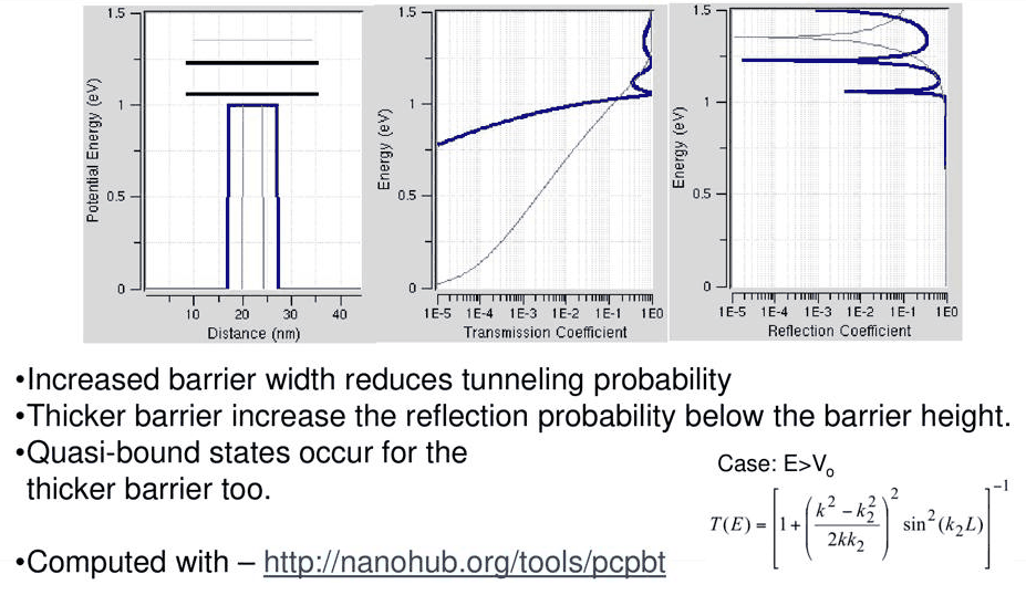
above the barrier: transmission below one, oscillating with \(k_2L\), and reaching one at quasi-bound states above the barrier
numerical observations with nanoHUB's PCPBT tool for a 1 eV barrier, thin and thick

In this notebook

computes the lecture's PCPBT plots (transmission and reflection of a 1 eV barrier, 4 nm and 10 nm wide) with open-nemo, compares them with the exact formula and with its two limits, locates the above-barrier resonances, and explores what the formula cannot do: a barrier with a heavier effective mass.

Run the notebookEvery number and figure on this page comes from it. Change it, rerun it, take it further.

Download .ipynb View on GitHub

Run it on your own machine

The notebook needs open-nemo (Python ≥ 3.10 and a C++20 compiler; BLAS/LAPACK).

git clone https://github.com/denphi/open-nemo.git && cd open-nemo
python3 -m venv .venv && source .venv/bin/activate
pip install -e ".[notebooks]"
jupyter lab From_Atoms_to_Devices/03_tunneling_and_bandstructure/06_2_single_barrier.ipynb

Code8 lines · cell 1

import numpy as np
import matplotlib.pyplot as plt
import opennemo as nemo
from opennemo.visualization import style

style.use(notebook=True)
H2M0 = nemo.core.units.HBAR2_2M0          # ħ²/2m₀ = 0.0381 eV nm²
EM = nemo.structures.materials.EffectiveMassMaterial

1. The exact transmission#

Lecture 6.1 reduced the single barrier to a 2×2 transfer matrix \(M = M_1M_2\) with \([A, B]^T = M[E, F]^T\). With \(F = 0\) the transmission is \(T = |E/A|^2 = 1/|M_{11}|^2\), and working out \(M_{11}\) ("a lot of analytical push-ups", in Klimeck's words, and a good exercise) gives, for an energy below the barrier top,

T(E) = \left[1 + \left(\frac{\gamma^2 + k^2}{2k\gamma}\right)^2 \sinh^2(\gamma L)\right]^{-1}, \qquad k = \frac{\sqrt{2mE}}{\hbar},\quad \gamma = \frac{\sqrt{2m(V_0 - E)}}{\hbar}.

The hyperbolic sine carries the exponential decay inside the barrier, governed by the barrier width \(L\) and the decay constant \(\gamma\). The form \(1/(1 + \text{something})\) shows that \(T\) can approach one when the something becomes small.

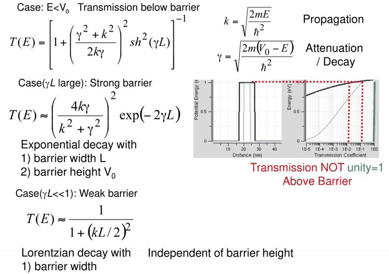
Slide 5: the exact transmission below the barrier and its two limits — Slide 5: the exact result, the strong-barrier limit (exponential in \(L\) and in \(\sqrt{V_0}\)) and the weak-barrier limit (a Lorentzian). The PCPBT plot compares a thin and a thick 1 eV barrier.

The lecture's PCPBT example is a 1 eV barrier with the GaAs effective mass \(0.067\,m_0\), 4 nm wide (thin) and 10 nm wide (thick). open-nemo computes \(T(E)\) of the same structures from the discretized Schrödinger equation with open boundaries. Above the barrier the same formula holds with \(\gamma \to ik_2\), \(k_2 = \sqrt{2m(E - V_0)}/\hbar\), so \(\sinh^2(\gamma L) \to -\sin^2(k_2L)\) and \((\gamma^2 + k^2)^2/\gamma^2 \to -(k^2 - k_2^2)^2/k_2^2\):

T(E) = \left[1 + \left(\frac{k^2 - k_2^2}{2kk_2}\right)^2 \sin^2(k_2L)\right]^{-1} = \left[1 + \frac{V_0^2\,\sin^2(k_2L)}{4E(E - V_0)}\right]^{-1}.

Code50 lines · cell 3

M, V0, DX, LEAD = 0.067, 1.0, 0.01, 5.0


def barrier(width, height=V0, mass=M, dx=DX):
    gaas = EM("GaAs", M, 12.9)
    bar = EM("barrier", mass, 12.9, conduction_band_edge=height)
    return nemo.Heterostructure1D(
        [nemo.Layer(gaas, LEAD), nemo.Layer(bar, width), nemo.Layer(gaas, LEAD)], spacing=dx
    )


def t_exact(E, L, V0=V0, m=M):
    # the single-barrier formula, below and above the barrier (complex γ covers both)
    k = np.sqrt(m * E / H2M0 + 0j)
    g = np.sqrt(m * (V0 - E) / H2M0 + 0j)
    return (1 / (1 + ((g**2 + k**2) / (2 * k * g)) ** 2 * np.sinh(g * L) ** 2)).real


E = np.concatenate([np.linspace(0.002, 0.999, 1500), np.linspace(1.001, 1.5, 1500)])
fig, axes = plt.subplots(1, 3, figsize=(13, 4.2), gridspec_kw={"width_ratios": [0.9, 1, 1]})
colours = {4.0: style.OPEN_NEMO, 10.0: style.sweep(4)[3]}
for L, lw in ((4.0, 1.0), (10.0, 2.2)):
    dev = barrier(L)
    T = nemo.Transport(dev.hamiltonian).transmission(E)
    print(
        f"L = {L:4.1f} nm: largest |ln(T open-nemo / T exact)| = "
        f"{np.abs(np.log(T / t_exact(E, L))).max():.1e};"
        f"  T at 0.02 eV = {np.interp(0.02, E, T):.1e}, at 0.5 eV = {np.interp(0.5, E, T):.2e},"
        f" at the top = {np.interp(V0, E, T):.3f}"
    )
    axes[0].plot(dev.x - dev.x.mean(), dev.band_edge, color=colours[L], lw=lw, label=f"{L:.0f} nm")
    axes[1].semilogx(T, E, color=colours[L], lw=lw)
    axes[2].semilogx(1 - T, E, color=colours[L], lw=lw)
    axes[1].semilogx(t_exact(E, L), E, ":", color=style.REFERENCE, lw=0.9)
axes[0].set(
    xlabel="distance from the centre (nm)",
    ylabel="potential energy (eV)",
    ylim=(-0.03, 1.55),
    title="1 eV barrier",
)
axes[0].legend(frameon=False, fontsize=8)
axes[1].set(
    xlabel="transmission T",
    ylabel="energy (eV)",
    xlim=(1e-5, 2),
    ylim=(0, 1.5),
    title="T(E) (dotted: formula)",
)
axes[2].set(xlabel="reflection R = 1 − T", xlim=(1e-5, 2), ylim=(0, 1.5), title="R(E)")
fig.tight_layout();

L =  4.0 nm: largest |ln(T open-nemo / T exact)| = 1.2e-04;  T at 0.02 eV = 8.6e-06, at 0.5 eV = 2.21e-03, at the top = 0.124
L = 10.0 nm: largest |ln(T open-nemo / T exact)| = 2.3e-04;  T at 0.02 eV = 1.2e-12, at 0.5 eV = 2.87e-08, at the top = 0.022

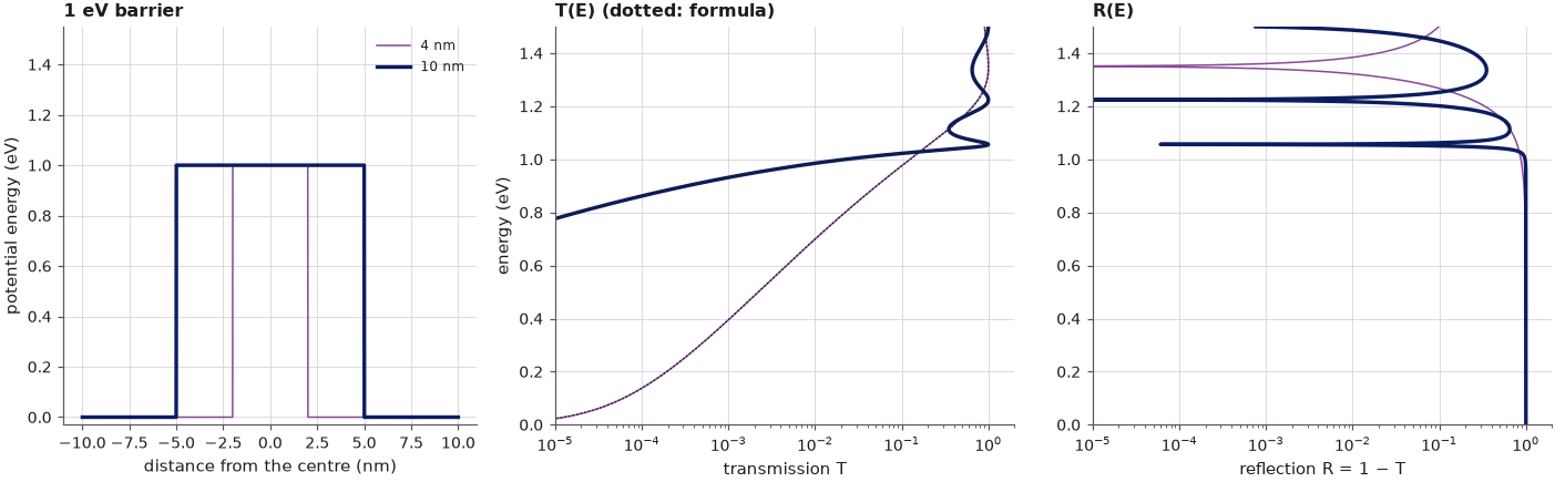
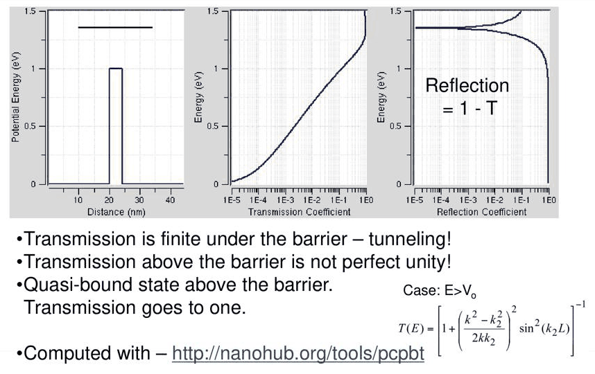
Figure computed by the notebook with open-nemo

The figure is the lecture's (slides 9 and 10, below), with the axes of PCPBT: energy upwards, transmission on a logarithmic scale. open-nemo and the formula agree to the small discretization error of the grid. Three observations, all impossible classically:

Tunneling. Below the barrier the transmission is finite. For the thin barrier it rises nearly exponentially with energy, from \(9\cdot10^{-6}\) at 0.02 eV to 0.12 at the top.
No unit transmission at the top. Classically \(T\) would jump from 0 to 1 at \(E = V_0\). Here it is 0.12 (thin) and 0.02 (thick) at the top, and above the top it reaches one only at isolated energies.
The thick barrier attenuates much more strongly below the top (\(3\cdot10^{-8}\) against \(2\cdot10^{-3}\) at 0.5 eV), and it also reflects more at and just above the top.

Slide 10: thin and thick barriers in PCPBT — Slide 10: PCPBT's result for the same two barriers (thin: thin line, thick: thick line). The open-nemo curves above reproduce it.

2. The strong barrier: exponential decay#

For \(\gamma L \gg 1\), \(\sinh(\gamma L) \approx e^{\gamma L}/2\) and the one in the bracket is negligible:

T(E) \approx \left(\frac{4k\gamma}{k^2 + \gamma^2}\right)^2 e^{-2\gamma L}.

The transmission falls exponentially with the barrier width \(L\) and, through \(\gamma \propto \sqrt{V_0 - E}\), with the barrier height. The prefactor depends on the energy only through \(k/\gamma\); it is at most 4 (at \(k = \gamma\)). The cell checks how quickly the limit becomes accurate, and shows both dependences with open-nemo.

Code33 lines · cell 5

def t_strong(E, L, V0=V0, m=M):
    k, g = np.sqrt(m * E / H2M0), np.sqrt(m * (V0 - E) / H2M0)
    return (4 * k * g / (k**2 + g**2)) ** 2 * np.exp(-2 * g * L)


Ec = 0.5
g = np.sqrt(M * (V0 - Ec) / H2M0)
print(f"E = {Ec} eV, V0 = {V0} eV: γ = {g:.3f} 1/nm, decay length 1/γ = {1 / g:.3f} nm")
print("  L (nm)   γL     T exact      T strong-barrier   relative error")
for L in (0.25, 0.5, 1.0, 2.0, 4.0, 10.0):
    te, ts = t_exact(Ec, L), t_strong(Ec, L)
    print(f"{L:7.2f}  {g * L:5.2f}   {te:.4e}   {ts:.4e}         {ts / te - 1:+.2e}")

widths = np.linspace(0.5, 10, 20)
heights = np.linspace(0.6, 2.0, 15)
t_w = [nemo.Transport(barrier(w, dx=0.02).hamiltonian).transmission([Ec])[0] for w in widths]
t_h = [nemo.Transport(barrier(4.0, h, dx=0.02).hamiltonian).transmission([Ec])[0] for h in heights]
fig, (a1, a2) = plt.subplots(1, 2, figsize=(11, 3.6))
a1.semilogy(widths, t_w, "o", color=style.OPEN_NEMO, ms=4, label="open-nemo")
a1.semilogy(widths, t_strong(Ec, widths), color=style.REFERENCE, lw=1, label="strong-barrier limit")
a1.set(xlabel="barrier width L (nm)", ylabel=f"T at E = {Ec} eV", title=f"{V0} eV barrier: exponential in L")
a2.semilogy(np.sqrt(heights - Ec), t_h, "o", color=style.OPEN_NEMO, ms=4, label="open-nemo")
a2.semilogy(
    np.sqrt(heights - Ec),
    [t_strong(Ec, 4.0, h) for h in heights],
    color=style.REFERENCE,
    lw=1,
    label="strong-barrier limit",
)
a2.set(xlabel="√(V₀ − E)  (eV^½)", ylabel=f"T at E = {Ec} eV", title="4 nm barrier: exponential in √(V₀ − E)")
for a in (a1, a2):
    a.legend(frameon=False, fontsize=8)
fig.tight_layout();

E = 0.5 eV, V0 = 1.0 eV: γ = 0.938 1/nm, decay length 1/γ = 1.066 nm
  L (nm)   γL     T exact      T strong-barrier   relative error
   0.25   0.23   9.4700e-01   2.5029e+00         +1.64e+00
   0.50   0.47   8.0880e-01   1.5661e+00         +9.36e-01
   1.00   0.94   4.6101e-01   6.1318e-01         +3.30e-01
   2.00   1.88   8.9731e-02   9.3998e-02         +4.76e-02
   4.00   3.75   2.2065e-03   2.2089e-03         +1.10e-03
  10.00   9.38   2.8665e-08   2.8665e-08         +1.43e-08

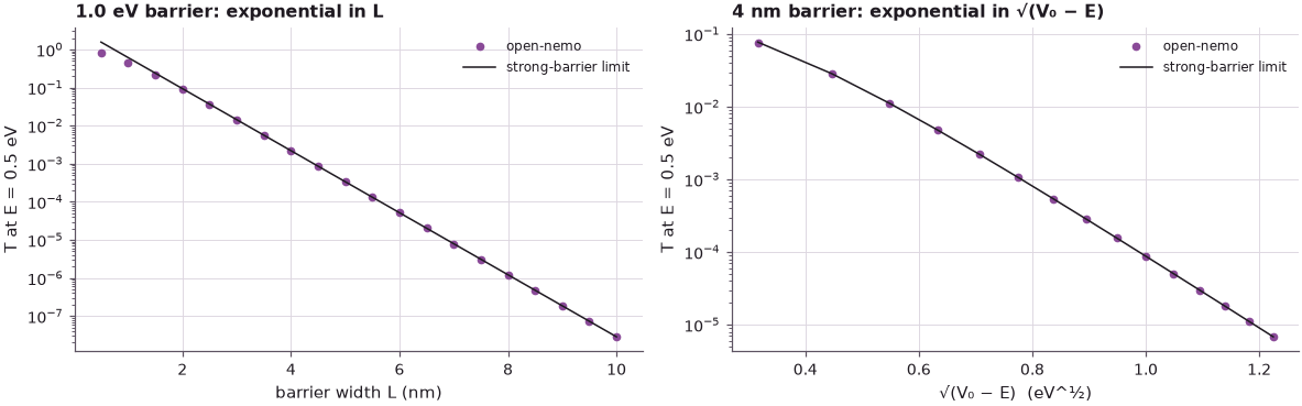
At \(\gamma L \approx 2\) the approximation is 5 % too high, at \(\gamma L \approx 4\) only 0.1 %, and it becomes exact quickly after that; for thin barriers it fails completely (it even exceeds one). Both plots are straight lines on the logarithmic scale: \(\ln T\) is linear in the width and linear in \(\sqrt{V_0 - E}\), the WKB-like dependence that makes tunnel currents so sensitive to oxide thickness and barrier height.

3. The weak barrier: a Lorentzian#

In the opposite limit, \(\gamma L \ll 1\), \(\sinh(\gamma L) \approx \gamma L\) and the bracket becomes \(1 + (k^2 + \gamma^2)^2L^2/4k^2\). Exactly at the barrier top (\(E = V_0\), \(\gamma = 0\)) the exact formula itself reduces to

T(V_0) = \frac{1}{1 + (kL/2)^2}, \qquad k = \sqrt{2mV_0}/\hbar,

a Lorentzian in the barrier width. The decay constant has dropped out, which is what the slide means by "independent of barrier height": there is no exponential suppression left, only the reflection caused by the jump of the wave number at the two interfaces, which grows with \(L\) as \(1/L^2\). The next cell compares how \(T\) falls with width at the top and halfway up.

Code20 lines · cell 7

L = np.linspace(0.2, 15, 40)
k_top = np.sqrt(M * V0 / H2M0)
t_top = [nemo.Transport(barrier(w, dx=0.02).hamiltonian).transmission([V0])[0] for w in L]
t_mid = [nemo.Transport(barrier(w, dx=0.02).hamiltonian).transmission([V0 / 2])[0] for w in L]
fig, ax = plt.subplots(figsize=(7.5, 3.8))
ax.loglog(L, t_top, "o", color=style.OPEN_NEMO, ms=4, label="open-nemo, E = V₀ (barrier top)")
ax.loglog(L, 1 / (1 + (k_top * L / 2) ** 2), color=style.REFERENCE, lw=1, label="Lorentzian 1/(1 + (kL/2)²)")
ax.loglog(L, t_mid, "s", color=style.sweep(4)[3], ms=4, label="open-nemo, E = V₀/2")
ax.set(
    xlabel="barrier width L (nm)",
    ylabel="T",
    ylim=(1e-12, 2),
    title=f"{V0} eV barrier: algebraic against exponential",
)
ax.legend(frameon=False, fontsize=8)
print(f"k at the barrier top = {k_top:.3f} 1/nm; Lorentzian half width L = 2/k = {2 / k_top:.2f} nm")
print(
    f"at L = 15 nm: T(V0) = {t_top[-1]:.3e} (Lorentzian {1 / (1 + (k_top * 15 / 2) ** 2):.3e}), T(V0/2) "
    f"= {t_mid[-1]:.1e}"
)

k at the barrier top = 1.326 1/nm; Lorentzian half width L = 2/k = 1.51 nm
at L = 15 nm: T(V0) = 1.001e-02 (Lorentzian 1.001e-02), T(V0/2) = 2.4e-12

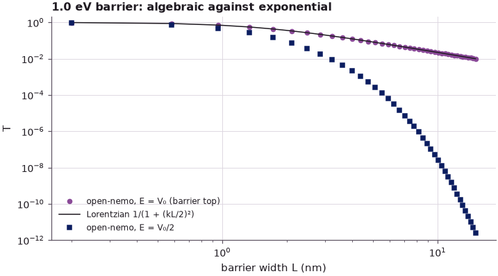
At the top the transmission falls only as \(1/L^2\): through a 15 nm barrier about one per cent still gets across, while halfway up the same barrier lets through less than \(10^{-10}\).

4. Above the barrier: oscillations and quasi-bound states#

Above the barrier the wave propagates inside it with \(k_2\), and the transmission

T(E) = \left[1 + \frac{V_0^2\,\sin^2(k_2L)}{4E(E - V_0)}\right]^{-1}

oscillates: it is one exactly when \(\sin(k_2L) = 0\), i.e. when the barrier holds an integer number of half wavelengths, \(k_2L = n\pi\), at

E_n = V_0 + n^2\,\frac{\hbar^2\pi^2}{2mL^2}.

The two interfaces act like the mirrors of a Fabry–Pérot resonator: the waves reflected at the two interfaces cancel when the round trip is a whole number of wavelengths. These resonances are quasi-bound states above the barrier, and they are not equally spaced: they follow the \(n^2\) of a particle in a box of width \(L\). Between them the reflection is finite; at them it vanishes, which on PCPBT's logarithmic reflection axis is a deep, narrow dip.

Slide 9: transmission and reflection of the thin barrier — Slide 9: the 4 nm barrier. The transmission reaches one at about 1.35 eV, where the reflection drops to zero.

Code20 lines · cell 9

from scipy.signal import find_peaks

Ea = np.linspace(1.0005, 2.5, 6000)
fig, (a1, a2) = plt.subplots(1, 2, figsize=(11, 4))
print(" L (nm)   n   E_n formula (eV)   T peak open-nemo (eV)   T at the peak   R minimum")
for L, c in ((4.0, style.OPEN_NEMO), (10.0, style.sweep(4)[3])):
    T = nemo.Transport(barrier(L).hamiltonian).transmission(Ea)
    peaks, _ = find_peaks(T)
    En = V0 + np.arange(1, 8) ** 2 * H2M0 * np.pi**2 / (M * L**2)
    for n, p in enumerate(peaks[:4], 1):
        print(f"{L:6.1f}   {n}   {En[n - 1]:12.4f}   {Ea[p]:16.4f}          {T[p]:.6f}     {1 - T[p]:.1e}")
    a1.plot(T, Ea, color=c, lw=1.1, label=f"L = {L:.0f} nm")
    a2.semilogx(1 - T, Ea, color=c, lw=1.1, label=f"L = {L:.0f} nm")
    a1.plot(np.ones_like(En[En < 2.5]), En[En < 2.5], "<", color=c, ms=6)
a1.set(
    xlabel="transmission T", ylabel="energy (eV)", xlim=(0, 1.05), title="above a 1 eV barrier (◂: k₂L = nπ)"
)
a2.set(xlabel="reflection R = 1 − T", xlim=(1e-7, 1), title="reflection: zeros at the resonances")
a1.legend(frameon=False, fontsize=8, loc="center left")
fig.tight_layout();

 L (nm)   n   E_n formula (eV)   T peak open-nemo (eV)   T at the peak   R minimum
   4.0   1         1.3508             1.3507          1.000000     6.9e-08
   4.0   2         2.4031             2.4030          1.000000     1.0e-09
  10.0   1         1.0561             1.0562          0.999955     4.5e-05
  10.0   2         1.2245             1.2245          1.000000     1.8e-07
  10.0   3         1.5051             1.5052          1.000000     8.5e-08
  10.0   4         1.8980             1.8979          1.000000     1.0e-07

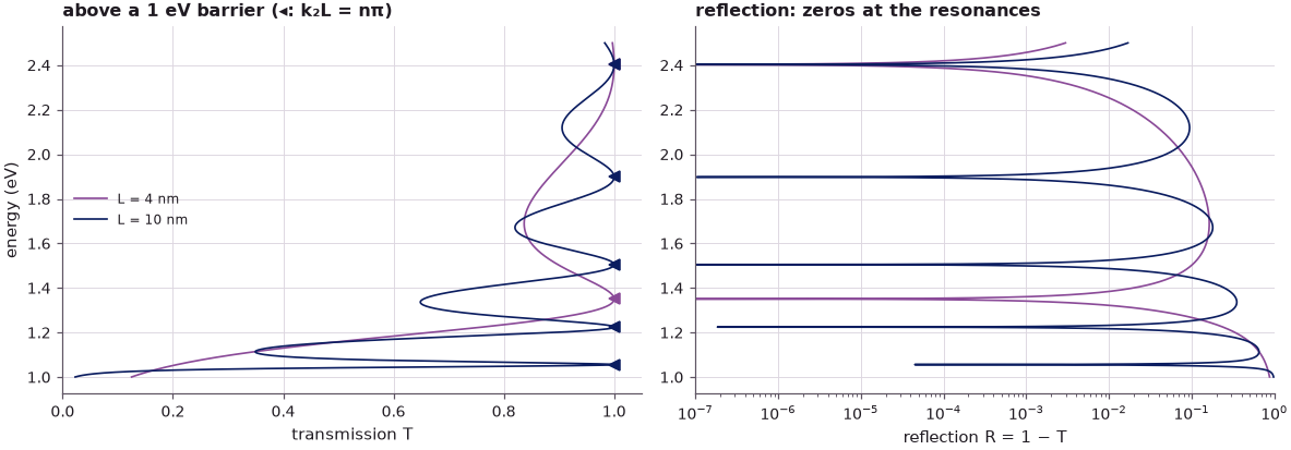
The peaks of open-nemo's transmission sit at the formula's \(E_n\) to the energy grid's resolution (0.25 meV), and there \(T = 1\) within \(5\cdot10^{-5}\); the largest deviation is the narrow first peak of the thick barrier, which the grid samples slightly off its top. The thin barrier has its first resonance 0.35 eV above the top, the thick one already at 56 meV, with the next at 0.22 and 0.50 eV above the top: the \(n^2\) spacing. Between the peaks the thick barrier reflects more, but its minima of \(T\) rise towards one with energy as \(V_0^2/4E(E - V_0)\) shrinks: far above the barrier the electron no longer notices it.

5. Exploration: a heavier barrier#

The formulas assume the same effective mass everywhere. In a real heterostructure the barrier material has its own mass (AlAs has about \(0.15\,m_0\), against GaAs's 0.067). open-nemo's grid handles this with the BenDaniel–Duke condition (continuity of \(\psi'/m\)), as the general transfer matrix of Lecture 6.1 does. A heavier barrier decays faster, \(\gamma \propto \sqrt{m_b}\), and it also changes the matching at the interfaces.

Code17 lines · cell 11

Eb = np.linspace(0.005, 1.5, 1500)
fig, ax = plt.subplots(figsize=(7.5, 4))
print(" barrier mass (m₀)   T at 0.5 eV    γ at 0.5 eV (1/nm)   first T = 1 above the top (eV)")
for mb, c in zip((0.067, 0.1, 0.15), style.sweep(3)):
    T = nemo.Transport(barrier(4.0, mass=mb, dx=0.02).hamiltonian).transmission(Eb)
    above = Eb > V0
    first = Eb[above][find_peaks(T[above])[0][0]]
    print(
        f"{mb:12.3f}       {np.interp(0.5, Eb, T):.3e}      {np.sqrt(mb * 0.5 / H2M0):8.3f}            "
        f"{first:.3f}"
    )
    ax.semilogx(T, Eb, color=c, lw=1.1, label=f"barrier mass {mb} m₀")
ax.axhline(V0, color=style.CONTEXT, ls=":", lw=0.8)
ax.set(
    xlabel="transmission T", ylabel="energy (eV)", xlim=(1e-6, 2), title="4 nm, 1 eV barrier, GaAs contacts"
)
ax.legend(frameon=False, fontsize=8);

 barrier mass (m₀)   T at 0.5 eV    γ at 0.5 eV (1/nm)   first T = 1 above the top (eV)
       0.067       2.207e-03         0.938            1.350
       0.100       4.024e-04         1.146            1.235
       0.150       4.559e-05         1.403            1.157

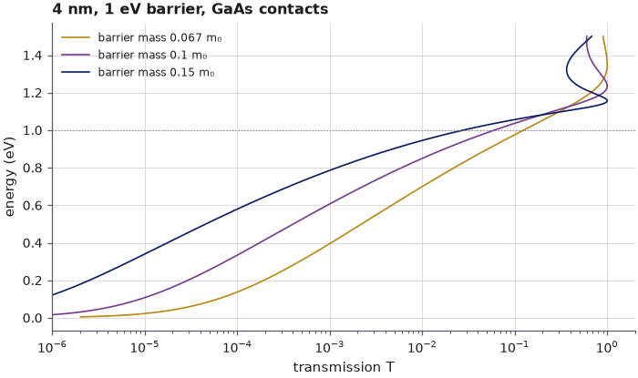
The heavier barrier transmits much less below the top (the exponent \(2\gamma L\) grows with \(\sqrt{m_b}\)), and its above-barrier resonance moves down towards the top, because the box energy \(\hbar^2\pi^2/2m_bL^2\) falls with the mass. The material, not only the geometry, sets the tunneling.

Summary#

\(T = 1/|M_{11}|^2\) of a single barrier has a closed form: \(\sinh^2(\gamma L)\) below the top, \(\sin^2(k_2L)\) above it. open-nemo's transmission reproduces it to the grid's discretization error.
Strong barrier (\(\gamma L \gtrsim 2\)): \(T \approx (4k\gamma/(k^2+\gamma^2))^2e^{-2\gamma L}\), exponential in width and in \(\sqrt{V_0 - E}\).
Weak barrier, or the barrier top: \(T = 1/(1 + (kL/2)^2)\), a Lorentzian in the width without exponential suppression.
The transmission is finite below the barrier (tunneling) and not one above it: interference between the two interfaces modulates it, with \(T = 1\) only at quasi-bound states \(k_2L = n\pi\).
The effective mass of the barrier enters both the decay and the resonances.

Exercises#

Plot the strong-barrier prefactor \((4k\gamma/(k^2+\gamma^2))^2\) against \(E/V_0\). Where is it largest, and why does it vanish at both ends?
Derive the above-barrier formula from the below-barrier one with \(\gamma = ik_2\), and check it numerically with t_exact and open-nemo at 1.2 eV for the 10 nm barrier.
For the 10 nm barrier, find the energy at which the minimum of \(T\) between two above-barrier resonances first exceeds 0.9.
Replace the GaAs contacts by a material with mass \(0.15\,m_0\) while keeping the barrier at \(0.067\,m_0\). Does the barrier transmit more or less at 0.5 eV, and why?