NEMO 3-D — strain: balls and springs

1. Lattice mismatch: an epitaxial layer deforms#

GaAs and InAs have the same zincblende structure, but InAs has a 7 % larger lattice constant (\(a_0\) = 0.6058 nm against \(a_s\) = 0.5653 nm for GaAs). When a thin InAs layer is grown on a thick GaAs substrate, the InAs bonds in the growth plane must match the substrate, so the layer is compressed in the plane. It responds by stretching along the growth direction. These deformations, and the islands (quantum dots) that form to relieve them, must be captured by the model.

In continuum elasticity, a cubic crystal biaxially strained in the (001) plane, \(\varepsilon_{xx} = \varepsilon_{yy} = \varepsilon_\parallel = (a_s - a_0)/a_0\), is free of stress along \(z\) (\(\sigma_{zz} = C_{12}\varepsilon_{xx} + C_{12}\varepsilon_{yy} + C_{11}\varepsilon_{zz} = 0\)), so

where \(C_{11}\) and \(C_{12}\) are the elastic constants of the layer. Klimeck stresses that in NEMO 3-D this formula is not used: the strain is a natural result of the interactions between the atoms.

2. The valence force field: atoms are balls, bonds are springs#

Each bond has a natural length \(d_0\) and each pair of bonds at an atom a natural angle \(\theta_0 = \arccos(-1/3) = 109.47°\). Deforming either costs energy:

with two constants per material: \(\alpha\) resists stretching and \(\beta\) resists bending. The sums run over every bond and every angle of the structure, with the constants of each bond type in a heterostructure. Keating's (1966) form, which open-nemo and NEMO 3-D use, writes the same physics with squared lengths and dot products,

which is rotation invariant and reduces to the slide's form for small deformations. More sophisticated force fields exist (NEMO 3-D has some), but two constants already give the three cubic elastic constants:

Since there are only two parameters, the three constants cannot all be fitted: Martin (1970) chose \(\alpha\) and \(\beta\) to reproduce \(C_{11}\) and \(C_{12}\) as well as possible, and \(C_{44}\) follows. open-nemo computes them from the strain energy of the relaxed bulk cell:

The relaxed-cell elastic constants agree with the closed-form Keating expressions. \(C_{11}\) and \(C_{12}\) are within 1–8 % of the measured values (slightly high), while \(C_{44}\) is 12 % low for GaAs and 21 % low for InAs. This is the price of a two-parameter model.

3. How NEMO 3-D uses the force field: strain is an output#

NEMO 3-D places every atom on an ideal lattice site, then minimizes the total spring energy over all atom positions (here with L-BFGS); the relaxed bond lengths and angles define the strain. The relaxed positions — not the strain — are passed on to the tight-binding Hamiltonian, which depends on every bond's length and direction. Splittings of degenerate bands then emerge from the deformations themselves.

The test case of slide 3: an InAs film, 6 cubic cells (3.6 nm) thick, on a GaAs substrate of 4 cells whose bottom cell is held fixed, periodic in the plane with the GaAs period and free at the top surface. The vertical lattice constant is read from the spacing of the In planes in the film.

The substrate keeps its bulk lattice constant and the film takes the GaAs period in the plane: \(\varepsilon_{xx} = \varepsilon_{yy} = -6.69\,\%\) comes out of the relaxed bonds, together with \(\varepsilon_{zz} = +7.17\,\%\) and no shear. The relaxed \(a_\perp\) = 0.6493 nm is 0.003 nm below the continuum value 0.6524 nm. At a mismatch of 7 % the difference is not an error of either model: the continuum formula is linear in the strain, while Keating's energy, written with squared lengths, is not. A sweep of the substrate lattice constant shows the two agree for small mismatch. Here the "substrate" is an InAs film whose in-plane period is set to \(a_s\), with only its bottom two atomic planes held.

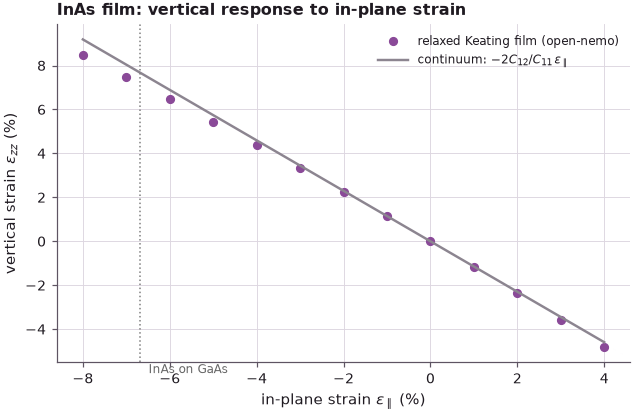
For strains of a per cent or two the relaxed film follows the continuum line; at large compression the force field gives a smaller vertical expansion, and under tension a larger contraction, than the linear law. The atomistic relaxation needs no such formula: it handles any geometry — a film, a pyramid, a random alloy — with the same two constants per bond.

4. Impact of strain on the electronic structure#

Strain changes bond lengths and angles, which shifts the band edges and lifts the degeneracy of the heavy-hole (HH) and light-hole (LH) bands at Γ. In continuum language this is described with deformation potentials (slide 6):

with \(a_c = -5.08\) eV, \(a_v = 1.0\) eV and \(b_v = -1.8\) eV for InAs. The first term of each line is the hydrostatic shift, proportional to the relative volume change; the \(b_v\) term responds to the tetragonal distortion and splits HH from LH. Klimeck's caveat: tight binding does not work this way. It sees only the displaced atoms, and these formulas serve to interpret its results and to check that it gives the right trends. Below, both are applied to bulk InAs strained biaxially in the (001) plane, from 0 to the pseudomorphic strain on GaAs, with \(\varepsilon_{zz} = -2(C_{12}/C_{11}) \varepsilon_\parallel\). The tight-binding model is sp3d5s* with spin–orbit coupling and the strain model of Boykin et al. (2002) (klimeck2002_sp3d5s: bond-length exponents of the two-centre integrals and strain-dependent on-site energies).

Both descriptions agree on the trends: the conduction band rises under compression, the valence degeneracy is lifted with the heavy hole on top, and both are of the order of a few hundred meV at the 6.7 % in-plane compression of InAs on GaAs. The numbers differ. The tight-binding model's own deformation potentials, obtained from small strains, are \(a_c = -6.32\) eV, \(a_v = 0.56\) eV and \(|b_v| = 1.18\) eV, not the slide's values; and at large strain the light hole, which is coupled to the split-off band by the strain (the spin–orbit splitting of InAs is only 0.39 eV), does not follow the linear formula at all: it bends back up. In a dot, where the strain varies from atom to atom, tight binding takes all of this into account without any formula.

5. Piezoelectric potential#

Zincblende has no inversion center, so shear strain polarizes it. To first order (slide 7),

with the piezoelectric constant \(e_{14}\) (\(-0.16\) C/m² for GaAs, \(-0.045\) C/m² for InAs). The slide also shows the second-order terms \(\mathbf{P}_2\) with constants \(B_{114}\), \(B_{124}\), \(B_{156}\), products of strain components. The polarization gives a bound charge density and, through Poisson's equation, a potential \(V_p\):

where \(\varepsilon_s\) is the static relative permittivity (sign conventions differ between authors; the slide writes the equation with the opposite sign). A (001) film has no shear strain and hence no piezoelectric field; a dot has shear strain along its edges. Below, the small pyramid of the previous lecture (InAs, base 9 nm, height 3.5 nm, on a wetting layer) is placed in a larger GaAs box of 26 × 26 × 14 cubic cells (14.7 × 14.7 × 7.9 nm, periodic), relaxed, its strain computed per atom against each atom's own material, \(\mathbf{P}_1\) put on the cations, and the potential solved on a grid of spacing \(a/2\), periodic in the plane and held at zero on the bottom and top faces.

The piezoelectric potential has the quadrupole pattern known from the literature: lobes of opposite sign along the two diagonals [110] and [1$\bar1$0] of the square base, strongest at the pyramid's corners and edges, where the shear strain is largest (up to 4.90 % here). On this plane, 1.1 nm above the base, the potential inside the dot is positive along [110] (about 9 mV) and negative along [1$\bar1$0] (about −4 mV), and the signs reverse just outside the base (−15 and +14 mV). Tens of millivolts are small compared with the band offsets, but comparable to the splitting of the p-like electron states, so the potential breaks the symmetry between [110] and [1$\bar1$0] that the square base alone would keep. NEMO 3-D adds \(-qV_p\) to the on-site energies of the tight-binding Hamiltonian, as the multi-scale chart of lecture 21.1 shows; later lectures of the course discuss its effect on dots.

Summary#

• Lattice mismatch makes an InAs layer on GaAs compress in the plane (\(\varepsilon_\parallel\) = −6.69 %) and expand vertically.
• The valence force field has two constants per material, \(\alpha\) for bond stretching and \(\beta\) for bond bending; they fix \(C_{11}\) and \(C_{12}\), while \(C_{44}\) comes out 12–21 % low.
• Minimizing the force-field energy over all atoms gives the strain as an output: the relaxed film has \(a_\perp\) = 0.6493 nm against 0.6524 nm from linear elasticity; the two agree at small mismatch.
• Tight binding of the strained crystal and deformation potentials agree on trends (CB up, HH above LH under compression) but not on numbers; the light hole is strongly nonlinear.
• Shear strain at the edges of a dot gives a piezoelectric polarization \(2e_{14}(\varepsilon_{yz}, \varepsilon_{xz}, \varepsilon_{xy})\) and a potential of tens of mV (−27 to +25 mV at the atoms of this small pyramid) with lobes of opposite sign along [110] and [1$\bar1$0].

Exercises#

1. Set \(\beta\) of InAs to zero in KEATING and recompute the elastic constants. What happens to \(C_{44}\), and why is a pure bond-stretching model unstable?
2. Change the film thickness NFILM to 2 and to 10 cells. Does \(a_\perp\) in the middle of the film change? Plot the In-plane spacing against height to see the surface and interface regions.
3. Repeat section 4 for tensile strain (\(\varepsilon_\parallel > 0\)). Which hole band is on top?
4. In section 5, use pz.zincblende_site_polarization(pyr, strain, order="second") to include the second-order terms of slide 7. How much does the potential change?

Further reading#

• Strained InAs/GaAs dot: relaxation and strain shifts of a dot's levels.
• Atomistic piezoelectric potential: the full piezoelectric chain, conventions and comparison with the literature.
• Strain types and directions and strained Si/Ge heterostructures.
• Dot strain profiles: NEMO 3-D strain benchmarks.
• Phonons and relaxation.
• Previous: multi-scale by design; next: sp3d5s* tight binding.
• P. N. Keating, Phys. Rev. 145, 637 (1966); R. M. Martin, Phys. Rev. B 1, 4005 (1970).
• T. B. Boykin, G. Klimeck, R. C. Bowen, F. Oyafuso, Phys. Rev. B 66, 125207 (2002) — the strain model of the tight-binding parameters.
• G. Klimeck et al., IEEE Trans. Electron Devices 54, 2090 (2007) — NEMO 3-D's strain and piezoelectric chain.