Lecture 23.7

Theory of stress and strain — from strain to band edges

In the lecture

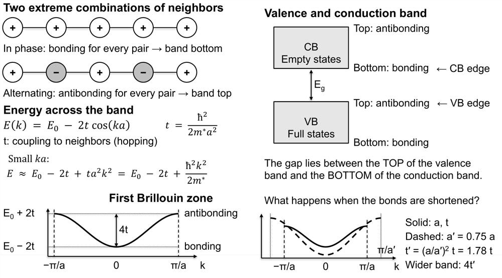
Inside a band the bottom is bonding and the top antibonding; shortening the bonds increases the coupling $t$ and widens the band.
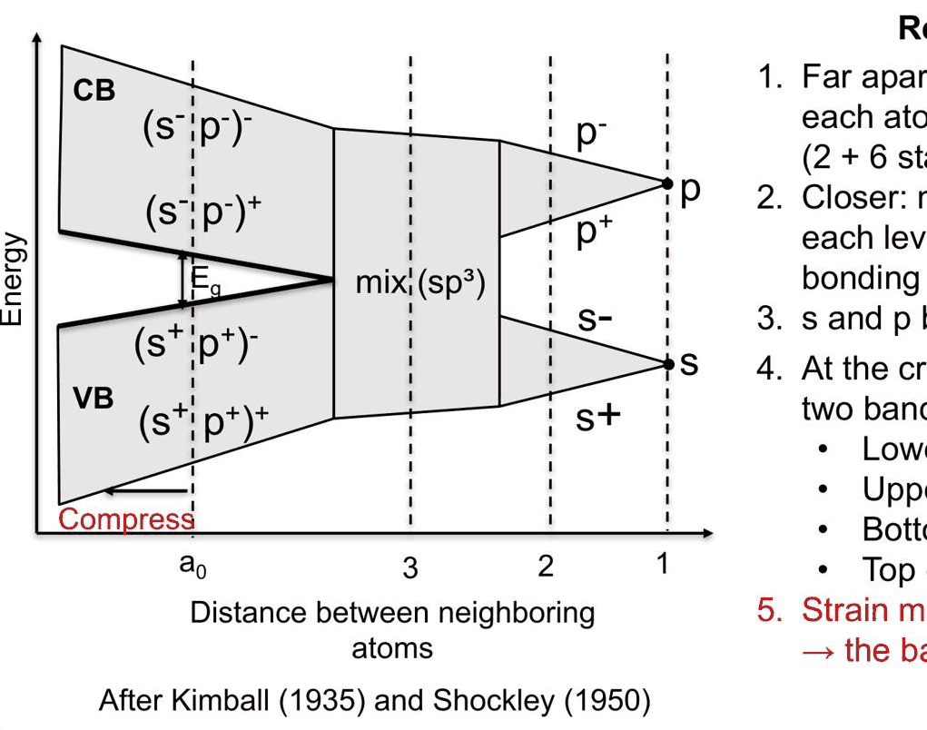
From atoms to bands (after Kimball and Shockley): s and p levels broaden, mix into sp³ hybrids and open the gap; strain moves the crystal left or right of $a_0$ and the band edges move.
Deformation potentials: a volume change shifts the edges, $\delta E = a\,\mathrm{Tr}\,\varepsilon$; for GaAs the gap rises by about 11 meV per kbar of pressure, as measured.
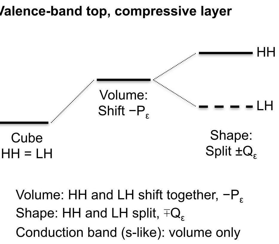
A shape change splits heavy and light holes (Bir–Pikus): $\delta E_\mathrm{HH} = -P_\varepsilon - Q_\varepsilon$, $\delta E_\mathrm{LH} = -P_\varepsilon + Q_\varepsilon$, with $Q_\varepsilon = b(\varepsilon_\perp - \varepsilon_\parallel)$.
GaAs under ±1 % biaxial strain and the worked example In${0.2}$Ga${0.8}$As on GaAs: shifts of tens of meV, comparable with the 200–400 meV barriers of heterostructure design.

In this notebook

You compute the band of a chain of s orbitals at two bond lengths with open-nemo's tight-binding builder, follow the sp³s* bands of silicon as the atoms are brought together, check the pressure coefficient of the GaAs gap, evaluate the Bir–Pikus shifts by hand and compare them with the 8-band k·p Hamiltonian (kp.bulk_hamiltonian, kp.gamma_edge_shifts), work through In${0.2}$Ga${0.8}$As on GaAs step by step, and compute the band-edge profile and subbands of a GaAs/In${0.2}$Ga${0.8}$As/GaAs quantum well with and without strain (kp.Heterostructure).

Run the notebookEvery number and figure on this page comes from it. Change it, rerun it, take it further.

Download .ipynb View on GitHub

Run it on your own machine

The notebook needs open-nemo (Python ≥ 3.10 and a C++20 compiler; BLAS/LAPACK).

git clone https://github.com/denphi/open-nemo.git && cd open-nemo
python3 -m venv .venv && source .venv/bin/activate
pip install -e ".[notebooks]"
jupyter lab From_Atoms_to_Devices/09_stress_and_strain/23_7_strain_to_band_edges.ipynb

Code10 lines · cell 1

import numpy as np
import matplotlib.pyplot as plt
import opennemo as nemo
from opennemo.visualization import style
import dataclasses
from opennemo.models import kp
from opennemo.solvers import elasticity as E
from opennemo.structures.structure import Structure

style.use(notebook=True)

1. Inside a band: bonding at the bottom, antibonding at the top#

The simplest crystal is a chain of atoms with one s orbital each, coupled to its neighbours by the hopping energy $t$. Two combinations of the orbitals are extreme. All orbitals in phase is bonding for every pair of neighbours and gives the bottom of the band; alternating signs is antibonding for every pair and gives the top. In between, the energy follows

E(k) = E_0 - 2t\cos ka ,

a band of width $4t$ across the Brillouin zone $-\pi/a \le k \le \pi/a$. Near the bottom, $E \approx E_0 - 2t + t a^2 k^2 = E_0 - 2t + \hbar^2k^2/2m^*$, so $t = \hbar^2/(2m^* a^2)$: this is how $t$ is calibrated from an effective mass. In a semiconductor the full bands are the valence bands, the empty ones the conduction bands; the gap lies between the top of the valence band, an antibonding state, and the bottom of the conduction band, a bonding state.

What happens when the bonds are shortened? In this model the coupling scales as $1/a^2$. For $a' = 0.75\,a$ it becomes $t' = (a/a')^2 t = 1.78\,t$, the band widens to $4t'$, and the Brillouin zone grows to $\pm\pi/a'$.

Slide 2: bonding and antibonding states of a chain, and a wider band for shorter bonds — Slide 2. In-phase (bonding) and alternating (antibonding) combinations of s orbitals form the bottom and top of the band $E = E_0 - 2t\cos ka$. Solid: spacing $a$ and coupling $t$; dashed: $a' = 0.75a$ with $t' = 1.78t$ and a wider band.

The chain can be built with open-nemo's Slater–Koster tight-binding builder from a one-orbital material (tb.single_band_material, whose hopping is $-t$), on a structure with a single period along $x$:

Code18 lines · cell 3

a, t = 0.5, 1.0                                                  # nm, eV
fig, ax = plt.subplots(figsize=(6.5, 3.8))
for ap, ls in ((a, "-"), (0.75 * a, "--")):
    tp = t * (a / ap) ** 2                                       # coupling scales as 1/a^2
    mat = nemo.models.tb.single_band_material(ap, onsite=0.0, hopping=-tp)
    chain = Structure(np.zeros((1, 3)), ["X"], np.array([[ap, 0.0, 0.0]]))
    h = nemo.models.tb.SlaterKoster(mat).build(chain)
    k = np.linspace(-np.pi / ap, np.pi / ap, 201)
    e = np.array([np.linalg.eigvalsh(h.dense(np.array([kk, 0.0, 0.0])))[0] for kk in k])
    err = np.abs(e - (-2 * tp * np.cos(k * ap))).max()
    ax.plot(k * a / np.pi, e, ls=ls, color=style.OPEN_NEMO, label=f"a' = {ap / a:.2f} a,  t' = {tp:.2f} t")
    print(f"a' = {ap / a:.2f} a: t' = {tp:.3f} eV, band from {e.min():+.3f} to {e.max():+.3f} eV "
          f"(width {e.max() - e.min():.3f} eV); max deviation from E0 − 2t cos ka: {err:.1e} eV")
ax.set_xlabel("k (π/a)")
ax.set_ylabel("E − E0 (eV)")
ax.set_title("A chain of s orbitals: shorter bonds, wider band")
ax.legend(fontsize=8)
plt.show()

a' = 1.00 a: t' = 1.000 eV, band from -2.000 to +2.000 eV (width 4.000 eV); max deviation from E0 − 2t cos ka: 0.0e+00 eV
a' = 0.75 a: t' = 1.778 eV, band from -3.556 to +3.556 eV (width 7.111 eV); max deviation from E0 − 2t cos ka: 0.0e+00 eV

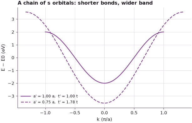
Figure computed by the notebook with open-nemo

The tight-binding chain reproduces $E_0 - 2t\cos ka$ to machine precision: a band 4 eV wide for $t = 1$ eV, 7.11 eV wide when the spacing shrinks to 0.75 $a$. The bonding bottom moves down and the antibonding top moves up. For a semiconductor this means that compressing the crystal pushes the top of the valence band (antibonding) and the bottom of the conduction band (bonding) in different directions, and the gap changes.

2. From atoms to bands#

Real semiconductors have s and p orbitals. Klimeck reads the classic picture of Kimball (1935) and Shockley (1950) from right to left, from atoms far apart to the crystal:

Far apart, each atom has an s and three p orbitals (2 + 6 states with spin) at their atomic energies.
Closer, neighbours interact and each level broadens into a band, bonding at the bottom and antibonding at the top.
Closer still, the s and p bands overlap and mix into sp³ hybrids.
At the crystal spacing $a_0$ a new gap has opened between two bands of 4 states per atom each: the lower, filled valence band and the upper, empty conduction band, each bonding at its bottom and antibonding at its top.
Strain moves the crystal left or right of $a_0$, and the band edges move.

Slide 7: s and p levels broadening into bands as the atoms approach — Slide 7. Energy against the distance between neighbouring atoms, after Kimball (1935) and Shockley (1950): s and p levels broaden, mix (sp³) and open the gap $E_g$ between valence band (VB) and conduction band (CB) at the crystal spacing $a_0$; compression moves the crystal to the left.

The same diagram can be computed. The cell below takes Vogl's sp³s* tight-binding model of silicon (an s, three p and an excited s* orbital per atom), scales the lattice by a factor $s$ and the couplings by $1/s^2$ (Harrison's scaling, as for the chain), and records the energy range of the valence bands (the lower four of the cell's ten) and of the conduction bands over the Brillouin zone.

Code24 lines · cell 5

si = nemo.structures.materials.load("vogl1983_sp3s")["Si"]
a0 = si.lattice_constant
rng = np.random.default_rng(0)
k_frac = np.vstack([(rng.random((120, 3)) - 0.5) * 4 * np.pi,                 # random k (units of 1/a)
                    np.outer(np.linspace(0, 1, 21), [2 * np.pi, 0, 0]),       # Γ–X
                    np.outer(np.linspace(0, 1, 11), [np.pi, np.pi, np.pi])])  # Γ–L

def band_ranges(scale):
    bonds = {key: [dataclasses.replace(b, v=tuple(np.array(b.v) / scale**2)) for b in bl]
             for key, bl in si.bonds.items()}
    m = dataclasses.replace(si, lattice_constant=a0 * scale, bonds=bonds)
    lat = nemo.structures.lattice.from_material(m)
    h = nemo.models.tb.SlaterKoster(m).build(nemo.structures.structure.bulk(lat))
    e = np.array([np.linalg.eigvalsh(h.dense(k / (a0 * scale))) for k in k_frac])
    return e[:, :4].min(), e[:, :4].max(), e[:, 4:].min(), e[:, 4:].max()

scales = np.linspace(0.85, 3.0, 44)
rng_e = np.array([band_ranges(s) for s in scales])
d = np.sqrt(3) / 4 * a0 * scales                                 # nearest-neighbour distance (nm)
gap = rng_e[:, 2] - rng_e[:, 1]
i0 = np.argmin(np.abs(scales - 1.0))
print(f"at a0 = {a0} nm (d = {10 * d[i0]:.3f} Å): VB {rng_e[i0, 0]:.2f} to {rng_e[i0, 1]:.2f} eV, "
      f"CB from {rng_e[i0, 2]:.2f} eV, gap {gap[i0]:.3f} eV")
print(f"the gap closes for d > {10 * d[np.argmax(gap <= 0)]:.2f} Å; onsite levels: {si.onsite['Si']}")

at a0 = 0.5431 nm (d = 2.352 Å): VB -12.50 to -0.00 eV, CB from 1.17 eV, gap 1.174 eV
the gap closes for d > 3.41 Å; onsite levels: {'s': -4.2, 'p': 1.715, 's*': 6.685}

Code17 lines · cell 6

fig, ax = plt.subplots(figsize=(7, 4.2))
ax.fill_between(10 * d, rng_e[:, 0], rng_e[:, 1], color=style.OPEN_NEMO, alpha=0.45, lw=0,
                label="valence bands")
ax.fill_between(10 * d, rng_e[:, 2], rng_e[:, 3], color=style.CONTEXT, alpha=0.45, lw=0,
                label="conduction bands")
for name, e0 in si.onsite["Si"].items():
    ax.axhline(e0, xmin=0.9, color="k", lw=1)
    ax.text(10 * d[-1] + 0.05, e0 + 0.3, name, va="bottom", fontsize=9)
ax.axvline(10 * d[i0], color="k", ls=":", lw=0.8)
ax.text(10 * d[i0] + 0.05, -15, "a0", fontsize=9)
ax.set_xlim(10 * d[0], 10 * d[-1] + 0.4)
ax.set_ylim(-16, 14)
ax.set_xlabel("distance between neighbouring atoms (Å)")
ax.set_ylabel("energy (eV)")
ax.set_title("Si sp³s*: from atomic levels to bands")
ax.legend(fontsize=8, loc="upper right", bbox_to_anchor=(0.88, 1.0))
plt.show()

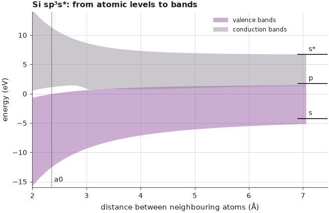
At large distance the bands shrink towards the atomic s, p and s* levels on the right. As the atoms approach, the bands broaden and overlap; the gap between the lower four and the upper six bands opens once the neighbour distance falls below 3.41 Å, and at the crystal spacing ($d = 2.352$ Å) silicon has an indirect gap of 1.174 eV in this model. Moving left (compression) or right (expansion) of $a_0$ moves both band edges. The model only scales all couplings uniformly, which is a hydrostatic strain; the next sections make this quantitative with deformation potentials, the numbers that experiments measure.

3. Deformation potentials: the volume shifts the edges#

Close to $a_0$ each band edge moves linearly with the relative volume change $\Delta V/V = \mathrm{Tr}\, \varepsilon$:

\delta E_c = a_c\,\mathrm{Tr}\,\varepsilon, \qquad \delta E_v = a_v\,\mathrm{Tr}\,\varepsilon, \qquad \delta E_g = (a_c - a_v)\,\mathrm{Tr}\,\varepsilon \equiv a\,\mathrm{Tr}\,\varepsilon .

The slopes $a_c$ and $a_v$ are the deformation potentials, in eV; the conduction and valence bands move at different rates because they are made of different orbitals. For GaAs, $a_c = -7.17$ eV and $a_v = +1.16$ eV (with the sign convention of the slides, in which a positive $a_v$ raises the valence band under expansion), so $a = -8.33$ eV: compression ($\mathrm{Tr}\,\varepsilon < 0$) opens the gap. An experiment checks this. Under hydrostatic pressure $p$, $\mathrm{Tr}\,\varepsilon = -p/B$ (case (a) of Lecture 23.4), so

\frac{\mathrm{d}E_g}{\mathrm{d}p} = -\frac{a}{B} \approx \frac{8.33\ \mathrm{eV}}{78.4\ \mathrm{GPa}} \approx 11\ \mathrm{meV/kbar},

and about 11 meV/kbar is what is measured for GaAs. Only the volume enters: pressure cannot tell $x$ from $y$ from $z$. The 8-band k·p Hamiltonian of open-nemo contains these deformation potentials (Vurgaftman's values); kp.gamma_edge_shifts returns the shifts of the conduction band and the top valence band at Γ for a given strain tensor.

Code12 lines · cell 8

gaas = kp.material("GaAs")
B = (gaas.c11 + 2 * gaas.c12) / 3
a_gap = gaas.ac - gaas.av
print(f"GaAs: a_c = {gaas.ac} eV, a_v = {gaas.av} eV, a = {a_gap:.2f} eV, B = {B:.1f} GPa")
print(f"dEg/dp = −a/B = {-a_gap / B * 1000:.1f} meV/GPa = {-a_gap / B * 100:.1f} meV/kbar")
p = 0.1                                                          # 1 kbar in GPa
dc, dv = kp.gamma_edge_shifts(gaas, -p / B / 3 * np.eye(3))      # hydrostatic: Tr ε = −p/B
print(f"8-band k·p at 1 kbar: δEc = {1000 * dc:+.2f} meV, δEv = {1000 * dv:+.2f} meV, "
      f"δEg = {1000 * (dc - dv):+.2f} meV")
dc1, dv1 = kp.gamma_edge_shifts(gaas, -0.01 / 3 * np.eye(3))      # volume change of −1 %
print(f"volume change −1 %: δEc = {1000 * dc1:+.1f} meV, δEv = {1000 * dv1:+.1f} meV, "
      f"δEg = {1000 * (dc1 - dv1):+.1f} meV")

GaAs: a_c = -7.17 eV, a_v = 1.16 eV, a = -8.33 eV, B = 78.4 GPa
dEg/dp = −a/B = 106.2 meV/GPa = 10.6 meV/kbar
8-band k·p at 1 kbar: δEc = +9.14 meV, δEv = -1.48 meV, δEg = +10.62 meV
volume change −1 %: δEc = +71.7 meV, δEv = -11.6 meV, δEg = +83.3 meV

The pressure coefficient is 10.6 meV/kbar, the "≈ 11 meV/kbar" of the slide and of experiment, and the k·p Hamiltonian gives the same number. A volume reduction of 1 % raises the conduction band by 71.7 meV and lowers the valence band by 11.6 meV, opening the gap by 83.3 meV: these are the numbers of the last column of the slide's table below (which labels it $\varepsilon_{xx,yy,zz}$; its values correspond to $\mathrm{Tr}\,\varepsilon = -1\,\%$, a third of a per cent along each axis).

4. A shape change splits heavy and light holes#

The conduction band bottom of GaAs is s-like, a sphere: only the volume matters. The valence band top is p-like, made of $p_x$, $p_y$ and $p_z$ orbitals. In a cube $x$, $y$ and $z$ are equivalent, the three have the same energy, and a volume change, which keeps the cube a cube, shifts all three together. Spin–orbit coupling splits two states off by $\Delta_\mathrm{so}$ and leaves four at the top, the heavy holes (HH), made of $p_x$ and $p_y$ only, and the light holes (LH), which contain $p_z$ with 2/3 weight; in the cube they are still degenerate.

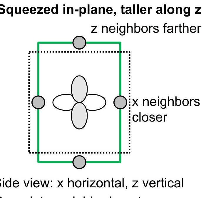
A thin layer squeezed in the plane and grown taller along $z$ is a tetragonal box. The orbitals along $x$ and $y$ see closer neighbours than the orbital along $z$, so they get a different energy, and HH and LH move apart. The splitting is proportional to the shape change, through the shear deformation potential $b$:

Q_\varepsilon = b\,(\varepsilon_\perp - \varepsilon_\parallel), \qquad E_\mathrm{HH} - E_\mathrm{LH} = -2Q_\varepsilon ,

with $b = -2.0$ eV for GaAs and $-1.8$ eV for InAs. In a compressed layer the heavy hole lies above the light hole; in a tensile layer the order is reversed.

Slide 11: the tetragonal box treats z differently from x and y — Slide 11. Squeezed in-plane and taller along $z$: the $x$ neighbours are closer and the $z$ neighbours farther, so $p_x$ and $p_z$ (side view) no longer have the same energy.

Putting the two effects together is the Bir–Pikus model (signs as in Chuang): a common shift from the volume and a splitting from the shape,

P_\varepsilon = -a_v\,\mathrm{Tr}\,\varepsilon, \qquad \delta E_\mathrm{HH} = -P_\varepsilon - Q_\varepsilon, \qquad \delta E_\mathrm{LH} = -P_\varepsilon + Q_\varepsilon, \qquad \delta E_c = a_c\,\mathrm{Tr}\,\varepsilon .

Slide 12: the Bir–Pikus model, a common shift and a splitting — Slide 12. Valence-band top of a compressive layer: from the cube (HH = LH), the volume shifts both by $-P_\varepsilon$, the shape splits them by $\mp Q_\varepsilon$.

For a (001) layer everything follows from $\varepsilon_\parallel$ (Lecture 23.5). The cell below works through the slide's seven steps for GaAs and evaluates them at $\varepsilon_\parallel = \pm 1\,\%$:

Code18 lines · cell 10

def bir_pikus(m, e_par):
    r = m.c12 / m.c11
    tr, shape = 2 * (1 - r) * e_par, -(1 + 2 * r) * e_par
    P, Q = -m.av * tr, m.b * shape
    return {"Tr": tr, "shape": shape, "dEc": m.ac * tr, "-P": -P, "Q": Q, "HH": -P - Q, "LH": -P + Q}

c = bir_pikus(gaas, 1.0)                                         # coefficients per unit ε∥
print("GaAs, coefficients of ε∥:")
for key, lab in (("Tr", "1. volume Tr ε"), ("shape", "2. shape ε⊥ − ε∥"), ("dEc", "3. conduction band (eV)"),
                 ("-P", "4. common VB shift −Pε (eV)"), ("Q", "5. splitting Qε (eV)"),
                 ("HH", "6. heavy holes (eV)"), ("LH", "7. light holes (eV)")):
    print(f"   {lab:30s} {c[key]:+.3f} ε∥")
print(f"\n{'':10s}{'δEc':>8s}{'δEHH':>8s}{'δELH':>8s}{'EHH−ELH':>9s}{'ΔEg':>8s}   (meV)")
for e_par in (-0.01, 0.01):
    bp = bir_pikus(gaas, e_par)
    gap = bp["dEc"] - max(bp["HH"], bp["LH"])
    print(f"ε∥ = {100 * e_par:+.0f} %{1000 * bp['dEc']:+8.1f}{1000 * bp['HH']:+8.1f}{1000 * bp['LH']:+8.1f}"
          f"{1000 * (bp['HH'] - bp['LH']):+9.1f}{1000 * gap:+8.1f}")

GaAs, coefficients of ε∥:
   1. volume Tr ε                 +1.073 ε∥
   2. shape ε⊥ − ε∥               -1.927 ε∥
   3. conduction band (eV)        -7.693 ε∥
   4. common VB shift −Pε (eV)    +1.245 ε∥
   5. splitting Qε (eV)           +3.854 ε∥
   6. heavy holes (eV)            -2.610 ε∥
   7. light holes (eV)            +5.099 ε∥

               δEc    δEHH    δELH  EHH−ELH     ΔEg   (meV)
ε∥ = -1 %   +76.9   +26.1   -51.0    +77.1   +50.8
ε∥ = +1 %   -76.9   -26.1   +51.0    -77.1  -127.9

The steps give the slide's coefficients: $\mathrm{Tr}\,\varepsilon = 1.07\,\varepsilon_\parallel$, shape $-1.93\,\varepsilon_\parallel$, $\delta E_c = -7.69$ eV $\varepsilon_\parallel$, $-P_\varepsilon = +1.24$ eV $\varepsilon_\parallel$, $Q_\varepsilon = +3.85$ eV $\varepsilon_\parallel$, and so $\delta E_\mathrm{HH} = -2.61$ eV $\varepsilon_\parallel$ and $\delta E_\mathrm{LH} = +5.10$ eV $\varepsilon_\parallel$. Coefficients of a few eV times strains of a per cent are shifts of tens of meV: at $\varepsilon_\parallel = -1\,\%$ the conduction band rises by 76.9 meV, the heavy hole by 26.1 meV and the light hole falls by 51.0 meV, so the gap opens by 50.8 meV; at +1 % the signs reverse and the gap, now set by the light hole, shrinks by 127.9 meV. Heterostructures are designed with barriers of 200–400 meV, so these shifts are anything but small.

The Bir–Pikus formulas are the strain terms of the k·p Hamiltonian at Γ, with one simplification: they neglect the coupling of the light hole to the split-off band (the slide estimates about 10 meV at 1 %). The 8-band Hamiltonian keeps it. Its eigenvalues at Γ, with and without strain, give the shifts of all bands; in (001) biaxial strain the heavy hole does not couple to anything and must agree exactly.

Code11 lines · cell 12

def kp_shifts(m, eps):
    e0 = np.linalg.eigvalsh(kp.bulk_hamiltonian(m, np.zeros(3)))
    e1 = np.linalg.eigvalsh(kp.bulk_hamiltonian(m, np.zeros(3), strain=eps))
    pairs = e1[::2]                                              # Kramers pairs: SO, VB, VB, CB
    return pairs[3] - e0[-1], pairs[1:3] - e0[2]                 # δEc, the two top valence pairs

print(f"{'':10s}{'δEc':>9s}{'VB pair 1':>11s}{'VB pair 2':>11s}   8-band k·p (meV)")
for e_par in (-0.01, 0.01):
    eps = np.diag([e_par, e_par, -2 * gaas.c12 / gaas.c11 * e_par])     # (001) biaxial strain
    dEc, vb = kp_shifts(gaas, eps)
    print(f"ε∥ = {100 * e_par:+.0f} %{1000 * dEc:+9.1f}{1000 * vb[0]:+11.1f}{1000 * vb[1]:+11.1f}")

                δEc  VB pair 1  VB pair 2   8-band k·p (meV)
ε∥ = -1 %    +76.9      -41.5      +26.1
ε∥ = +1 %    -76.9      -26.1      +58.7

The conduction band (±76.9 meV) and the heavy hole agree with Bir–Pikus exactly: at −1 % the upper valence pair is the heavy hole at +26.1 meV, at +1 % the lower pair is the heavy hole at −26.1 meV. The light hole comes out at −41.5 meV instead of −51.0 meV under compression, and at +58.7 meV instead of +51.0 meV under tension: its coupling to the split-off band pushes it up by 9.5 and 7.7 meV, the size of correction the slide warns about.

The slide's comparison of biaxial and hydrostatic strain becomes a pair of plots: the band edges against $\varepsilon_\parallel$ for a (001) layer, and against $\varepsilon_{xx} = \varepsilon_{yy} = \varepsilon_{zz}$ for a uniform compression or expansion.

Code26 lines · cell 14

eps_scan = np.linspace(-0.01, 0.01, 21)
fig, (ax1, ax2) = plt.subplots(1, 2, figsize=(10, 4), sharey=True)
for e in eps_scan:
    dEc, vb = kp_shifts(gaas, np.diag([e, e, -2 * gaas.c12 / gaas.c11 * e]))
    ax1.plot([100 * e] * 3, 1000 * np.r_[dEc, vb], "o", ms=3, color=style.CONTEXT)
    dEc, vb = kp_shifts(gaas, e * np.eye(3))
    ax2.plot([100 * e] * 3, 1000 * np.r_[dEc, vb], "o", ms=3, color=style.CONTEXT)
bp = bir_pikus(gaas, eps_scan)
ax1.plot(100 * eps_scan, 1000 * bp["dEc"], color=style.OPEN_NEMO, label="CB")
ax1.plot(100 * eps_scan, 1000 * bp["HH"], color=style.REFERENCE, label="HH")
ax1.plot(100 * eps_scan, 1000 * bp["LH"], "--", color=style.REFERENCE, label="LH")
ax2.plot(100 * eps_scan, 1000 * gaas.ac * 3 * eps_scan, color=style.OPEN_NEMO, label="CB")
ax2.plot(100 * eps_scan, 1000 * gaas.av * 3 * eps_scan, color=style.REFERENCE, label="HH = LH")
ax1.plot([], [], "o", ms=3, color=style.CONTEXT, label="8-band k·p")
ax1.set_xlabel("in-plane strain ε∥ (%)")
ax1.set_ylabel("band-edge shift (meV)")
ax1.set_title("Biaxial (001): compressive ← → tensile")
ax2.set_xlabel("ε_xx = ε_yy = ε_zz (%)")
ax2.set_title("Hydrostatic")
ax1.legend(fontsize=8)
ax2.legend(fontsize=8)
for ax in (ax1, ax2):
    ax.axhline(0, color="k", lw=0.5)
    ax.axvline(0, color="k", lw=0.5)
plt.tight_layout()
plt.show()

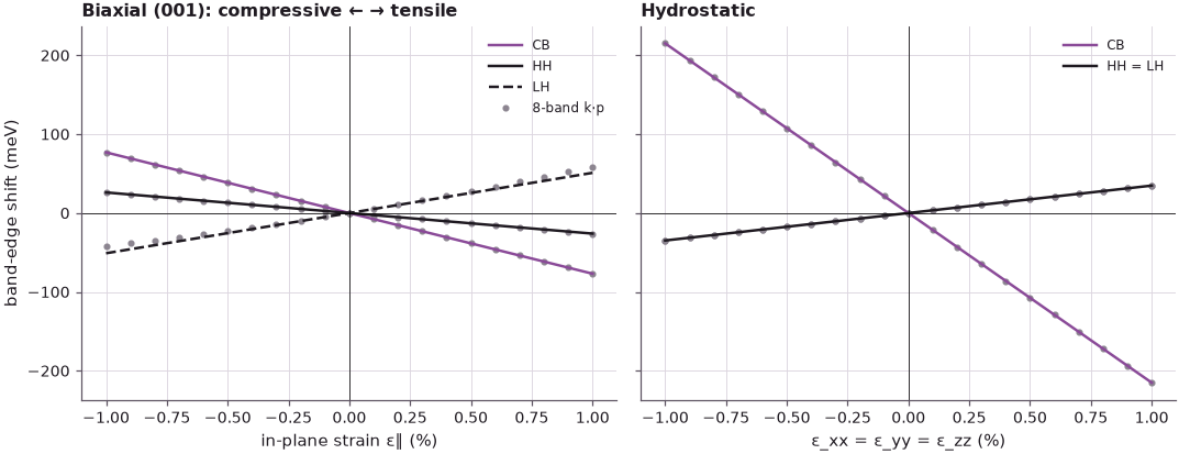
Under biaxial strain the heavy and light holes cross at zero strain: compression lifts the heavy hole, tension the light hole. Because the top valence band changes character at zero strain, the gap opens by 50.8 meV at 1 % compression but closes by 127.9 meV at 1 % tension. Under hydrostatic strain the two holes stay together (both lines are the same) and the gap simply opens under compression; with the same strain along all three axes the volume changes three times as much as in-plane, so the shifts are larger. Lines: Bir–Pikus; dots: 8-band k·p, which bends the light hole near the split-off band.

5. Worked example: In${0.2}$Ga${0.8}$As on GaAs (001)#

The lecture's example puts everything together. The parameters of the alloy are interpolated linearly between GaAs and InAs (Lecture 23.6) except the band gap, which bows (by 0.477 eV in Vurgaftman's compilation) and is taken from the measured alloy, 1.132 eV at 300 K.

Code18 lines · cell 16

inas = kp.material("InAs")
alloy_v = kp.material("InGaAs", x=0.2)                           # Vurgaftman: bowed gap, a and C linear
lin = lambda f: 0.8 * getattr(gaas, f) + 0.2 * getattr(inas, f)
alloy = dataclasses.replace(alloy_v, ac=lin("ac"), av=lin("av"), b=lin("b"),
                            valence_band_offset=lin("valence_band_offset"))
print(f"{'':12s}{'GaAs':>9s}{'InAs':>9s}{'In0.2Ga0.8As':>14s}")
for f, lab, sc in (("lattice_constant", "a0 (Å)", 10), ("ac", "ac (eV)", 1), ("av", "av (eV)", 1),
                   ("b", "b (eV)", 1), ("band_gap", "Eg (eV)", 1)):
    print(f"{lab:12s}{sc * getattr(gaas, f):9.3f}{sc * getattr(inas, f):9.3f}{sc * getattr(alloy, f):14.3f}")
print(f"{'C12/C11':12s}{gaas.c12 / gaas.c11:9.3f}{inas.c12 / inas.c11:9.3f}{alloy.c12 / alloy.c11:14.3f}")
e_par = gaas.lattice_constant / alloy.lattice_constant - 1
bp = bir_pikus(alloy, e_par)
print(f"\nε∥ = {100 * e_par:.2f} %, ε⊥ = {100 * -2 * alloy.c12 / alloy.c11 * e_par:+.2f} %, "
      f"Tr ε = {100 * bp['Tr']:.2f} %, ε⊥ − ε∥ = {100 * bp['shape']:+.2f} %")
print(f"δEc = {1000 * bp['dEc']:+.0f} meV, −Pε = {1000 * bp['-P']:+.0f} meV, Qε = {1000 * bp['Q']:+.0f} meV, "
      f"δEHH = {1000 * bp['HH']:+.0f} meV, δELH = {1000 * bp['LH']:+.0f} meV, "
      f"HH–LH splitting {1000 * (bp['HH'] - bp['LH']):.0f} meV")
print(f"gap {alloy.band_gap:.3f} eV → {alloy.band_gap + bp['dEc'] - bp['HH']:.3f} eV")

                 GaAs     InAs  In0.2Ga0.8As
a0 (Å)          5.653    6.058         5.734
ac (eV)        -7.170   -5.080        -6.752
av (eV)         1.160    1.000         1.128
b (eV)         -2.000   -1.800        -1.960
Eg (eV)         1.422    0.354         1.132
C12/C11         0.464    0.543         0.475

ε∥ = -1.41 %, ε⊥ = +1.34 %, Tr ε = -1.48 %, ε⊥ − ε∥ = +2.76 %
δEc = +100 meV, −Pε = -17 meV, Qε = -54 meV, δEHH = +37 meV, δELH = -71 meV, HH–LH splitting 108 meV
gap 1.132 eV → 1.195 eV

The layer is squeezed by 1.41 % in the plane and stretched by 1.34 % along $z$: a modest volume reduction of 1.48 % and a shape change of +2.76 %. The conduction band rises by 100 meV because the volume shrinks; the common valence shift is −17 meV and the splitting term −54 meV, so the heavy hole rises by 37 meV and the light hole falls by 71 meV, 108 meV below it. The gap opens from 1.132 eV to 1.195 eV, still well below the 1.422 eV of GaAs: the layer is a quantum well. As in Section 4, the 8-band Hamiltonian agrees for the conduction band and the heavy hole and moves the light hole:

Code3 lines · cell 18

eps_layer = kp.biaxial_strain(alloy, gaas.lattice_constant)
dEc, vb = kp_shifts(alloy, eps_layer)
print(f"8-band k·p: δEc = {1000 * dEc:+.1f} meV, HH = {1000 * vb[1]:+.1f} meV, LH = {1000 * vb[0]:+.1f} meV")

8-band k·p: δEc = +100.1 meV, HH = +37.3 meV, LH = -50.8 meV

With the split-off coupling the light hole lies 50.8 meV below its unstrained energy instead of 71 meV: at a shape change of 2.8 % the "≈ 10 meV per per cent" correction amounts to about 20 meV. The heavy hole (+37.3 meV) and conduction band (+100.1 meV) are as before.

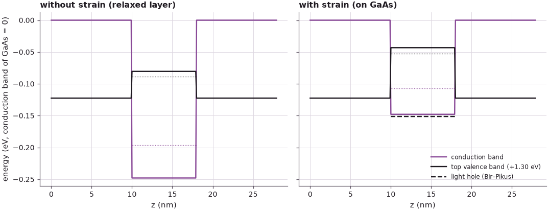
6. The GaAs / In${0.2}$Ga${0.8}$As / GaAs quantum well#

What matters for a device is the band alignment against the GaAs barriers. The valence band offset is interpolated linearly: InAs lies 0.21 eV above GaAs. Without strain (a relaxed layer, which cannot actually be grown on GaAs) the well would be deep for electrons and shallow for holes. With the strain of the pseudomorphic layer, the conduction band rises and the heavy hole rises, and the light hole sinks below the GaAs valence band.

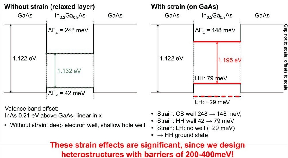
Slide 21: the GaAs/In0.2Ga0.8As/GaAs heterostructure with and without strain — Slide 21. Without strain: $\Delta E_c = 248$ meV, $\Delta E_v = 42$ meV. With strain: $\Delta E_c = 148$ meV, a heavy-hole well of 79 meV, and no light-hole well (−29 meV): the hole ground state is a heavy hole.

kp.Heterostructure builds the 8-band Hamiltonian of a layer stack on a grid. Given a substrate, it strains every layer pseudomorphically to it and adds the strain terms; without one, the layers are relaxed. The band-edge profile below is that of an 8 nm well between 10 nm GaAs barriers; the subbands are the confined states at $k_\parallel = 0$.

Code27 lines · cell 20

stack = [kp.Layer(gaas, 10.0), kp.Layer(alloy, 8.0), kp.Layer(gaas, 10.0)]
fig, axs = plt.subplots(1, 2, figsize=(10, 4), sharey=True)
for ax, sub, title in zip(axs, (None, gaas), ("without strain (relaxed layer)", "with strain (on GaAs)")):
    hs = kp.Heterostructure(stack, spacing=0.1, substrate=sub)
    ec, ev = hs.band_edges
    z = np.arange(len(ec)) * 0.1
    mid = len(ec) // 2
    e_el = hs.subbands(np.zeros((1, 2)), num=2)[0]
    e_h = hs.subbands(np.zeros((1, 2)), num=4, near=ev.max())[0]
    dEc, dEv = ec[0] - ec[mid], ev[mid] - ev[0]
    ax.plot(z, ec - ec[0], color=style.OPEN_NEMO, label="conduction band")
    ax.plot(z, ev - ec[0] + 1.30, color=style.REFERENCE, label="top valence band (+1.30 eV)")
    if sub is not None:
        lh = ev[0] + dEv - (bp["HH"] - bp["LH"])                    # LH edge in the well (Bir–Pikus)
        ax.hlines(lh - ec[0] + 1.30, 10, 18, color=style.REFERENCE, ls="--", label="light hole (Bir–Pikus)")
    ax.hlines(e_el[0] - ec[0], 10, 18, color=style.OPEN_NEMO, lw=0.8, ls=":")
    ax.hlines(np.max(e_h) - ec[0] + 1.30, 10, 18, color=style.REFERENCE, lw=0.8, ls=":")
    ax.set_title(title)
    ax.set_xlabel("z (nm)")
    print(f"{title:32s} ΔEc = {1000 * dEc:.1f} meV, ΔEv = {1000 * dEv:.1f} meV, gap in the well "
          f"{ec[mid] - ev[mid]:.4f} eV;  e1 {1000 * (e_el[0] - ec[mid]):.1f} meV above the well bottom, "
          f"top hole level {1000 * (ev[mid] - np.max(e_h)):.1f} meV below the well top")
axs[0].set_ylabel("energy (eV, conduction band of GaAs = 0)")
axs[1].legend(fontsize=8, loc="lower right")
plt.tight_layout()
plt.show()
print(f"light-hole offset with strain (Bir–Pikus): {1000 * (dEv - (bp['HH'] - bp['LH'])):.0f} meV")

without strain (relaxed layer)   ΔEc = 248.1 meV, ΔEv = 42.0 meV, gap in the well 1.1324 eV;  e1 51.8 meV above the well bottom, top hole level 8.2 meV below the well top
with strain (on GaAs)            ΔEc = 147.9 meV, ΔEv = 79.3 meV, gap in the well 1.1953 eV;  e1 40.6 meV above the well bottom, top hole level 9.6 meV below the well top

light-hole offset with strain (Bir–Pikus): -29 meV

The computation reproduces the slide. Without strain the electron well is 248.1 meV deep and the hole well 42.0 meV. With strain the electron well shrinks to 147.9 meV, the heavy-hole well deepens to 79.3 meV, and the light hole sees a barrier of 29 meV instead of a well, so the hole ground state is a heavy hole. The gap in the well opens from 1.1324 to 1.1953 eV. Strain changes the band offsets of this structure by 100 meV, half of a typical 200–400 meV design barrier.

One caveat on parameters. The slide, and the cell above, interpolate the deformation potentials and the valence band offset linearly. Vurgaftman's compilation, which kp.material("InGaAs", x=0.2) uses directly, bows both ($a_c = -7.17$ eV, and a valence offset 0.061 eV higher at $x = 0.2$):

Code8 lines · cell 22

for name, mat in (("linear (slide)", alloy), ("Vurgaftman bowing", alloy_v)):
    out = []
    for sub in (None, gaas):
        ec, ev = kp.Heterostructure([kp.Layer(gaas, 10.0), kp.Layer(mat, 8.0), kp.Layer(gaas, 10.0)],
                                    spacing=0.1, substrate=sub).band_edges
        out.append((1000 * (ec[0] - ec[len(ec) // 2]), 1000 * (ev[len(ev) // 2] - ev[0])))
    print(f"{name:18s} ac = {mat.ac:+.2f} eV, VBO = {mat.valence_band_offset:+.3f} eV:  "
          f"ΔEc {out[0][0]:.1f} → {out[1][0]:.1f} meV,  ΔEv {out[0][1]:.1f} → {out[1][1]:.1f} meV")

linear (slide)     ac = -6.75 eV, VBO = -0.758 eV:  ΔEc 248.1 → 147.9 meV,  ΔEv 42.0 → 79.3 meV
Vurgaftman bowing  ac = -7.17 eV, VBO = -0.697 eV:  ΔEc 187.3 → 80.9 meV,  ΔEv 102.8 → 140.1 meV

With the bowed parameters the electron well is 187.3 meV without strain and 80.9 meV with it, the hole well 102.8 and 140.1 meV: strain still moves the offsets by 106 meV and 37 meV, but the absolute depths depend on parameters that are less certain than the strain theory itself. The lecturer's point stands either way: the volume shifts the band edges, the shape splits the heavy and light holes, and in strained heterostructures both effects are as large as the band offsets being designed.

Summary#

In a band the bottom is bonding, the top antibonding; shorter bonds mean larger coupling ($t' = 1.78\,t$ for $a' = 0.75\,a$) and wider bands. In Si sp³s*, the gap opens below a neighbour distance of 3.41 Å and is 1.174 eV at $a_0$.
The volume shifts the edges: $\delta E = a\,\mathrm{Tr}\,\varepsilon$; GaAs has $a = -8.33$ eV and a pressure coefficient of 10.6 meV/kbar (measured ≈ 11 meV/kbar).
The shape splits heavy and light holes: $Q_\varepsilon = b(\varepsilon_\perp - \varepsilon_\parallel)$, $\delta E_\mathrm{HH,LH} = -P_\varepsilon \mp Q_\varepsilon$. GaAs at $\varepsilon_\parallel = -1\,\%$: CB +76.9, HH +26.1, LH −51.0 meV; the 8-band k·p model agrees for CB and HH and moves the LH by up to 10 meV through the split-off band.
In${0.2}$Ga${0.8}$As on GaAs: δEc = +100 meV, HH +37 meV, LH −71 meV, gap 1.132 → 1.195 eV. In a GaAs well the electron confinement drops from 248 to 148 meV, the heavy-hole well grows from 42 to 79 meV, and the light hole is not confined.

Exercises#

Repeat the worked example for In${0.3}$Ga${0.7}$As. Is the light hole confined now? How thick could such a layer be grown (Lecture 23.6)?
Compute the band edges of GaAs grown on an In${0.2}$Ga${0.8}$As substrate (tensile strain). Which hole is on top, and by how much?
Vary the well width of Section 6 from 4 to 12 nm and plot the electron and heavy-hole ground-state energies. Compare the strained and unstrained wells.
Build GaAs with a tight-binding model (nemo.models.tb.SlaterKoster(material, spin=True, strain="bond_length") on the klimeck2002_sp3d5s set), apply $\varepsilon_\parallel = -1\,\%$, and compare its band-edge shifts at Γ with the Bir–Pikus values.