Lecture 11.5

Asymmetric RTDs with charge accumulation and depletion

In the lecture

the sequential-tunneling picture of an RTD with different emitter and collector barriers: the well fills when the emitter barrier is the more transparent one and empties when it is the less transparent one
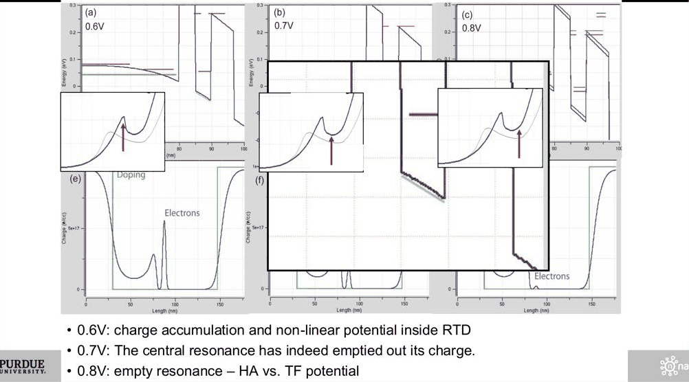
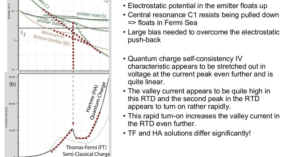
forward bias (thin barrier on the emitter side): charge accumulation, strong electrostatic push-back, non-linear resonance traces, an I–V stretched to higher voltages and currents, and a large difference between the Thomas–Fermi and Hartree models
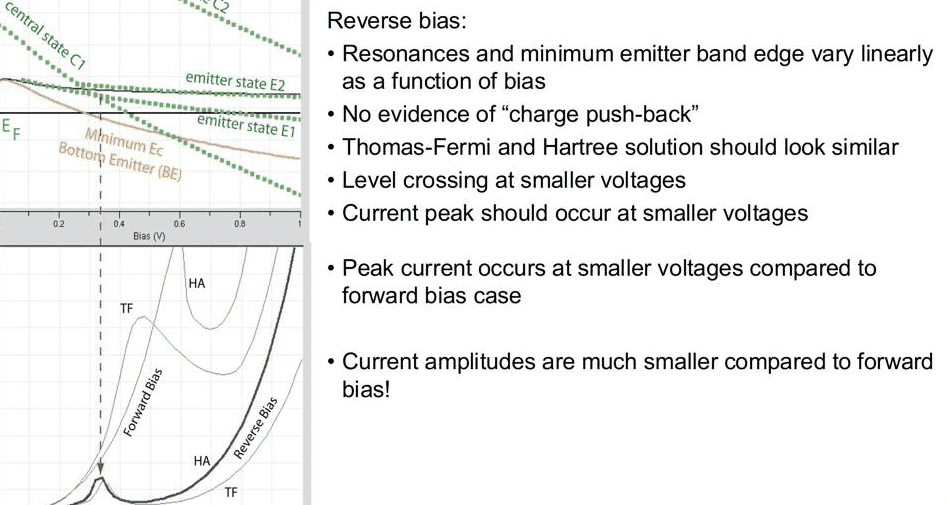
reverse bias (thick barrier on the emitter side): an empty well, resonances that move linearly with bias, Thomas–Fermi and Hartree results that nearly agree, and a smaller peak current at a smaller voltage
experimental tests on InGaAs/InAlAs RTDs (DRC 1997) with systematic variations of spacers, wells and barrier asymmetry
why the bias dependence of the tunneling rates makes simple analytic formulas unreliable

In this notebook

builds an RTD with a 5 nm emitter barrier and a 7 nm collector barrier, and its mirror image for reverse bias; it compares the Thomas–Fermi (nemo.thomas_fermi_iv) and Hartree (nemo.hartree_iv) I–V curves, band diagrams and resonance traces in both directions, the sheet charge in the well against the current, estimates the tunneling rates from resonance widths, and varies the collector barrier thickness to produce a systematic I–V asymmetry.

Run the notebookEvery number and figure on this page comes from it. Change it, rerun it, take it further.

Download .ipynb View on GitHub

Run it on your own machine

The notebook needs open-nemo (Python ≥ 3.10 and a C++20 compiler; BLAS/LAPACK).

git clone https://github.com/denphi/open-nemo.git && cd open-nemo
python3 -m venv .venv && source .venv/bin/activate
pip install -e ".[notebooks]"
jupyter lab From_Atoms_to_Devices/06_resonant_tunneling_diodes/11_5_asymmetric_rtds.ipynb

Code8 lines · cell 1

import numpy as np
import matplotlib.pyplot as plt
import opennemo as nemo
from opennemo.visualization import style

style.use(notebook=True)
H2M0 = nemo.core.units.HBAR2_2M0          # ħ²/2m₀ = 0.0381 eV nm²
EM = nemo.structures.materials.EffectiveMassMaterial

1. Sequential tunneling through two different barriers#

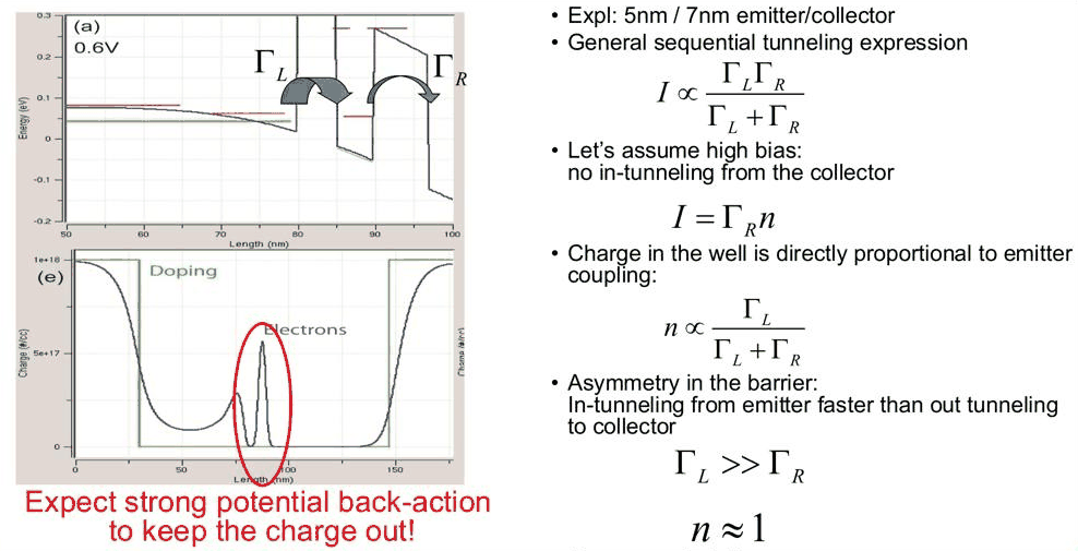
Treat the RTD as a single level in the well, coupled to the emitter at a rate $\Gamma_L/\hbar$ and to the collector at a rate $\Gamma_R/\hbar$ ($\Gamma_L$, $\Gamma_R$ are the partial widths of the resonance, in eV). With an occupation $n$ of the level (between 0 and 1), the rate equation $\dot n = \Gamma_L (f_L - n)/\hbar - \Gamma_R (n - f_R)/\hbar$ gives in steady state, with the level below the emitter Fermi level ($f_L = 1$) and far above the collector Fermi level ($f_R = 0$, no tunneling in from the collector):

n = \frac{\Gamma_L}{\Gamma_L + \Gamma_R}, \qquad I = \frac{e}{\hbar}\,\Gamma_R\, n = \frac{e}{\hbar}\,\frac{\Gamma_L \Gamma_R}{\Gamma_L + \Gamma_R}.

The current is symmetric in $\Gamma_L$ and $\Gamma_R$, but the charge is not. If the emitter barrier is the thinner one, $\Gamma_L \gg \Gamma_R$ and $n \to 1$: electrons come in faster than they leave and the well is full. The negative charge raises the potential in the well, and this electrostatic back-action pushes the resonance up, trying to keep the charge out. If the structure is reversed, $\Gamma_L \ll \Gamma_R$ and $n \to 0$: the well is empty and the electrostatics barely notices it.

Slide 3: an RTD with a 5 nm emitter and a 7 nm collector barrier, with the sequential tunneling formulas — Slide 3. An RTD with 5 nm emitter and 7 nm collector barriers at 0.6 V (top: conduction band, bottom: doping and electron density). The sequential-tunneling estimate gives $n \approx 1$ for $\Gamma_L \gg \Gamma_R$; a strong potential back-action is expected.

A quick estimate of the two rates: in a symmetric double barrier each barrier contributes half of the resonance width, so $\Gamma_{5} = w_{5/5}/2$ and $\Gamma_{7} = w_{7/7}/2$, where $w_{b/b}$ is the full width at half maximum of the first resonance of a flat-band GaAs/Al${0.3}$Ga${0.7}$As double barrier with two $b$ nm barriers and a 5 nm well. nemo.resonances returns these widths directly.

Code27 lines · cell 5

x_al = 0.3
gaas = EM("GaAs", 0.067, 12.9, conduction_band_edge=0.0)
algaas = EM("Al0.3Ga0.7As", 0.067 + 0.083 * x_al, 12.9 - 2.84 * x_al, conduction_band_edge=0.324)


def gamma_single(b):
    """Partial width (eV) of one b-nm barrier: half the width of a symmetric b/5/b double barrier."""
    layers = [
        nemo.Layer(gaas, 10),
        nemo.Layer(algaas, b),
        nemo.Layer(gaas, 5),
        nemo.Layer(algaas, b),
        nemo.Layer(gaas, 10),
    ]
    r = nemo.resonances(nemo.Heterostructure1D(layers, spacing=0.25), emax=0.3)
    return r["energy"][0], r["width"][0] / 2


(E5, G5), (E7, G7) = gamma_single(5.0), gamma_single(7.0)
print(
    f"5 nm barrier: Gamma = {G5 * 1e6:.2f} ueV;  7 nm barrier: Gamma = {G7 * 1e6:.3f} ueV "
    f"(C1 at {E5 * 1e3:.1f} and {E7 * 1e3:.1f} meV)"
)
print(f"ratio Gamma_5 / Gamma_7 = {G5 / G7:.1f}")
print(f"forward (5 nm emitter barrier): n = {G5 / (G5 + G7):.3f}")
print(f"reverse (7 nm emitter barrier): n = {G7 / (G5 + G7):.3f}")
print(f"sequential current factor G5*G7/(G5+G7) = {G5 * G7 / (G5 + G7) * 1e6:.3f} ueV in both directions")

5 nm barrier: Gamma = 46.64 ueV;  7 nm barrier: Gamma = 2.236 ueV (C1 at 84.1 and 84.1 meV)
ratio Gamma_5 / Gamma_7 = 20.9
forward (5 nm emitter barrier): n = 0.954
reverse (7 nm emitter barrier): n = 0.046
sequential current factor G5*G7/(G5+G7) = 2.134 ueV in both directions

Two extra nanometres of barrier reduce the partial width by more than an order of magnitude, so this simple picture predicts a nearly full well in forward bias and a nearly empty one in reverse bias, with the same current in both directions. The self-consistent calculations below show that only the first half of this prediction survives: the charge changes the potential, and the potential changes the rates.

2. The device in forward and reverse bias#

The device is the realistic-doping RTD of lectures 11.2–11.4 with thicker, unequal barriers: 30 nm GaAs contacts doped to $10^{18}$ cm$^{-3}$, 50 nm spacers at $10^{15}$ cm$^{-3}$, a 5 nm GaAs well, and Al${0.3}$Ga${0.7}$As barriers of 5 nm and 7 nm, at 300 K. Electrons always enter from the left contact, which is the emitter. Forward bias is the structure as built (5 nm barrier on the emitter side); reverse bias is simulated by mirroring the layer stack (7 nm barrier on the emitter side). Both use the reservoir relaxation of 6.6 meV; the Hartree calculation uses the quantum charge over both spacers, quantum_charge=(-200, 200), as in lecture 11.4.

Code29 lines · cell 7

def make_rtd(b_emitter, b_collector, well=5.0):
    layers = [
        nemo.Layer(gaas, 30, donors=1e18, name="emitter contact"),
        nemo.Layer(gaas, 50, donors=1e15, name="emitter spacer"),
        nemo.Layer(algaas, b_emitter, name="emitter barrier"),
        nemo.Layer(gaas, well, name="well"),
        nemo.Layer(algaas, b_collector, name="collector barrier"),
        nemo.Layer(gaas, 50, donors=1e15, name="collector spacer"),
        nemo.Layer(gaas, 30, donors=1e18, name="collector contact"),
    ]
    return nemo.Heterostructure1D(layers, spacing=0.25, terminal_layers=(2, 2))


T, XB1 = 300, 80.0
V = np.round(np.arange(0.0, 0.8001, 0.02), 3)
RES = (0.0066, 0.0066, "exponential", (-1, 0))
runs = {}
for name, (bl, br) in {"forward": (5.0, 7.0), "reverse": (7.0, 5.0)}.items():
    d = make_rtd(bl, br)
    well = (d.x > XB1 + bl) & (d.x < XB1 + bl + 5.0)
    tf = nemo.thomas_fermi_iv(d, V, T, charge="all")
    ha = nemo.hartree_iv(d, V, T, quantum_charge=(-200, 200))
    runs[name] = dict(d=d, bl=bl, br=br, well=well, tf=tf, ha=ha)
    print(
        f"{name}: {d.num_sites} sites, Hartree converged at all biases: {bool(np.all(ha['converged']))}, "
        f"max iterations {int(np.max(ha['iterations']))}"
    )
EF = float(np.atleast_1d(runs["forward"]["tf"]["mu_left"])[0])
print(f"emitter Fermi level {EF * 1e3:.1f} meV above the contact band edge")

forward: 708 sites, Hartree converged at all biases: True, max iterations 6
reverse: 708 sites, Hartree converged at all biases: True, max iterations 3
emitter Fermi level 41.9 meV above the contact band edge

3. Current–voltage characteristics#

The current is computed by NEGF with reservoir relaxation on each self-consistent potential. The function first_peak returns the first local maximum of $J(V)$.

Code24 lines · cell 9

def first_peak(J):
    return next(i for i in range(1, len(J) - 1) if J[i] >= J[i - 1] and J[i] > J[i + 1])


peaks = {}
for name, r in runs.items():
    for model in ("tf", "ha"):
        J = r[model]["current_density"]
        k = first_peak(J)
        peaks[name, model] = (V[k], J[k])
        valley = J[k:].min()
        print(
            f"{name:8s} {'Thomas-Fermi' if model == 'tf' else 'Hartree':12s}: peak {J[k]:6.0f} A/cm^2 at "
            f"{V[k]:.2f} V, valley {valley:5.0f} A/cm^2 at {V[k + np.argmin(J[k:])]:.2f} V"
        )

fig, axs = plt.subplots(1, 2, figsize=(11, 4), sharey=True)
for ax, name in zip(axs, runs):
    ax.plot(V, runs[name]["tf"]["current_density"], **style.series("reference"), label="Thomas–Fermi")
    ax.plot(V, runs[name]["ha"]["current_density"], **style.series(lw=2), label="Hartree")
    bl, br = runs[name]["bl"], runs[name]["br"]
    ax.set(xlabel="Bias (V)", title=f"{name} bias ({bl:.0f} nm / {br:.0f} nm barriers)")
    ax.legend()
axs[0].set_ylabel("Current density (A/cm$^2$)");

forward  Thomas-Fermi: peak    333 A/cm^2 at 0.48 V, valley   148 A/cm^2 at 0.70 V
forward  Hartree     : peak    521 A/cm^2 at 0.64 V, valley   436 A/cm^2 at 0.72 V
reverse  Thomas-Fermi: peak     59 A/cm^2 at 0.34 V, valley    23 A/cm^2 at 0.46 V
reverse  Hartree     : peak     92 A/cm^2 at 0.34 V, valley    34 A/cm^2 at 0.46 V

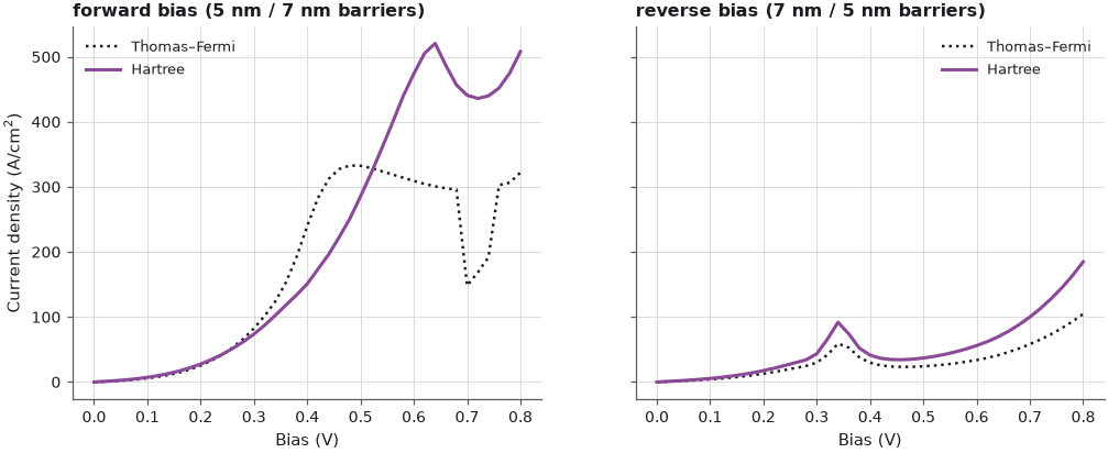
Figure computed by the notebook with open-nemo

The two directions behave very differently, as in the lecture:

Forward bias. The Hartree peak (521 A/cm$^2$ at 0.64 V) sits at a much higher voltage and a higher current than the Thomas–Fermi peak (333 A/cm$^2$ at 0.48 V), and the Hartree curve rises almost linearly up to it. The valley is shallow and high in the Hartree model (436 A/cm$^2$, against 148 A/cm$^2$), and the current turns on again quickly after it. The quantum charge piled up in the well holds the resonance up.
Reverse bias. Both models give the peak at 0.34 V, with 59 and 92 A/cm$^2$. The peak occurs at a much smaller voltage than in forward bias and the Hartree peak current is 5.7 times smaller.

The forward/reverse asymmetry of the peak current contradicts the sequential formula of section 1, which is symmetric in $\Gamma_L$ and $\Gamma_R$: the rates are not fixed numbers but depend on the bias and on the charge.

Slide 12: resonance traces and I–V in reverse bias compared with forward bias — Slide 12. Reverse bias in the lecture: (a) resonance and emitter band-edge traces that vary linearly with bias, (b) the I–V curves of forward and reverse bias, each in the Thomas–Fermi (TF) and Hartree (HA) models. The reverse-bias peak is at a smaller voltage and has a much smaller current.

4. Band diagrams around the forward peak#

The lecture shows the forward-bias band diagrams at 0.6 V (charge accumulation and a non-linear potential inside the RTD), at 0.7 V (the resonance has emptied) and at 0.8 V (empty resonance, Thomas–Fermi and Hartree potentials nearly equal again). The same sequence for this device is shown below at the Hartree peak, before it and after it. The horizontal lines mark the central resonance C1 in each model; the lower panels show the electron density.

Code31 lines · cell 13

def c1(device, u, bl, br):
    """Energy and width of the central resonance: the narrowest state located between the barriers."""
    r = nemo.resonances(device, potential=u, emax=0.35, reservoir=RES)
    m = (r["x0"] > XB1 + bl - 1) & (r["x0"] < XB1 + bl + 6) & (r["width"] < 5e-3)
    return (r["energy"][m][0], r["width"][m][0]) if m.any() else (np.nan, np.nan)


f = runs["forward"]
d, x = f["d"], f["d"].x
kp = int(np.argmin(abs(V - peaks["forward", "ha"][0])))
show = [V[kp] - 0.08, V[kp], 0.80]
fig, axs = plt.subplots(2, 3, figsize=(12, 6), sharex=True, sharey="row")
for j, v in enumerate(show):
    i = int(np.argmin(abs(V - v)))
    for model, color, lab in (("tf", style.REFERENCE, "Thomas–Fermi"), ("ha", style.OPEN_NEMO, "Hartree")):
        u = f[model]["potential"][i]
        e, w = c1(d, u, 5.0, 7.0)
        axs[0, j].plot(x, d.band_edge + u, color=color, lw=1.8, label=lab)
        axs[0, j].hlines(e, XB1 + 5, XB1 + 10, color=color, lw=2.5)
        axs[1, j].semilogy(x, f[model]["electron_density"][i], color=color, lw=1.5)
        print(
            f"{V[i]:.2f} V {lab:12s}: C1 = {e * 1e3:6.1f} meV, J = {f[model]['current_density'][i]:5.0f} "
            "A/cm^2, "
            f"well sheet density {f[model]['electron_density'][i][f['well']].sum() * 0.25e-7:.1e} cm^-2"
        )
    axs[0, j].axhline(EF, color=style.CONTEXT, ls=":", lw=1)
    axs[0, j].set(title=f"forward, {V[i]:.2f} V", xlim=(55, 115), ylim=(-0.45, 0.45))
    axs[1, j].set(xlabel="Position (nm)", ylim=(1e14, 3e19))
axs[0, 0].set_ylabel("Energy (eV)")
axs[1, 0].set_ylabel("$n$ (cm$^{-3}$)")
axs[0, 0].legend(loc="lower left");

0.56 V Thomas–Fermi: C1 =   38.8 meV, J =   319 A/cm^2, well sheet density 9.7e+08 cm^-2
0.56 V Hartree     : C1 =   65.5 meV, J =   399 A/cm^2, well sheet density 1.9e+11 cm^-2
0.64 V Thomas–Fermi: C1 =   23.0 meV, J =   301 A/cm^2, well sheet density 5.6e+08 cm^-2
0.64 V Hartree     : C1 =   53.2 meV, J =   521 A/cm^2, well sheet density 2.1e+11 cm^-2
0.80 V Thomas–Fermi: C1 =   -6.8 meV, J =   322 A/cm^2, well sheet density 1.8e+08 cm^-2
0.80 V Hartree     : C1 =  -13.7 meV, J =   508 A/cm^2, well sheet density 3.9e+10 cm^-2

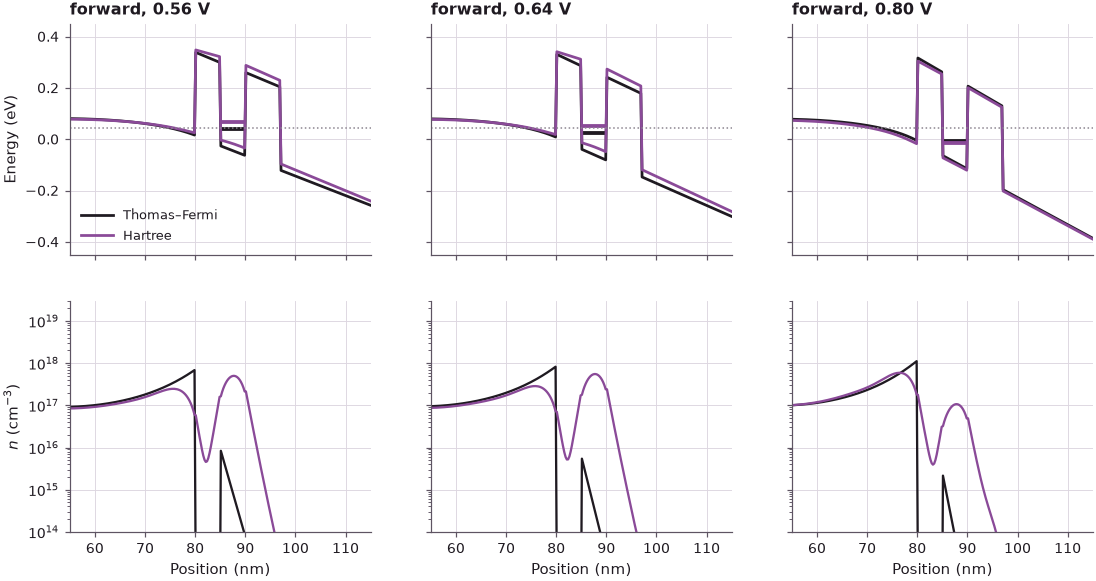
At 0.56 V and at the peak (0.64 V) the Hartree well holds a sheet density of about $2\times10^{11}$ cm$^{-2}$, more than two orders of magnitude above the semiclassical charge of the Thomas–Fermi model ($10^{9}$ cm$^{-2}$ and less), which has no knowledge of the non-equilibrium filling. The Hartree conduction band inside the double barrier is bent upward and C1 sits about 27–30 meV above its Thomas–Fermi position. The emitter accumulation layer in front of the first barrier is smaller in the Hartree model, so less bias drops across the emitter side and more across the collector side, which raises the current. At 0.80 V C1 has fallen to the emitter band bottom, the well charge is down by a factor of five to $3.9\times10^{10}$ cm$^{-2}$, and the two potentials nearly coincide.

Slide 6: band diagrams and charge distributions at 0.6, 0.7 and 0.8 V in forward bias — Slide 6. The lecture's forward-bias band diagrams and charge densities at 0.6 V (charge accumulation, non-linear potential inside the RTD), 0.7 V (the central resonance has emptied) and 0.8 V (empty resonance; Hartree and Thomas–Fermi potentials compared).

5. Resonance traces: push-back in forward bias, linear motion in reverse bias#

Tracing C1 and the bottom of the emitter notch (the lowest conduction-band energy in front of the emitter barrier) against bias shows the push-back directly. Energies are measured from the emitter contact band edge; the dotted line is the emitter Fermi level.

Code33 lines · cell 17

VT = V
traces = {}
for name, r in runs.items():
    d, bl, br = r["d"], r["bl"], r["br"]
    notch = (d.x > XB1 - 20) & (d.x < XB1)
    for model in ("tf", "ha"):
        idx = [int(np.argmin(abs(V - v))) for v in VT]
        traces[name, model] = dict(
            c1=np.array([c1(d, r[model]["potential"][i], bl, br) for i in idx]),
            bottom=np.array([(d.band_edge + r[model]["potential"][i])[notch].min() for i in idx]),
        )

fig, axs = plt.subplots(1, 2, figsize=(11, 4), sharey=True)
for ax, name in zip(axs, runs):
    for model, color, lab in (("tf", style.REFERENCE, "Thomas–Fermi"), ("ha", style.OPEN_NEMO, "Hartree")):
        t = traces[name, model]
        ax.plot(VT, t["c1"][:, 0], "o-", ms=3, color=color, label=f"C1, {lab}")
        ax.plot(VT, t["bottom"], "--", color=color, label=f"emitter bottom, {lab}")
    ax.axhline(EF, color=style.CONTEXT, ls=":")
    ax.set(xlabel="Bias (V)", title=f"{name} bias", ylim=(-0.12, 0.22))
axs[0].set_ylabel("Energy (eV)")
axs[0].legend(fontsize=8)

for name in runs:
    for model in ("tf", "ha"):
        e = traces[name, model]["c1"][:, 0]
        ok = VT <= 0.3
        slope = np.polyfit(VT[ok], e[ok], 1)[0]
        cross = VT[np.argmax(e < EF)]
        print(
            f"{name:8s} {model}: dC1/dV below 0.3 V = {slope:.3f} eV/V, C1 below the emitter Fermi level "
            f"from {cross:.2f} V"
        )

forward  tf: dC1/dV below 0.3 V = -0.338 eV/V, C1 below the emitter Fermi level from 0.56 V
forward  ha: dC1/dV below 0.3 V = -0.302 eV/V, C1 below the emitter Fermi level from 0.66 V
reverse  tf: dC1/dV below 0.3 V = -0.370 eV/V, C1 below the emitter Fermi level from 0.48 V
reverse  ha: dC1/dV below 0.3 V = -0.373 eV/V, C1 below the emitter Fermi level from 0.44 V

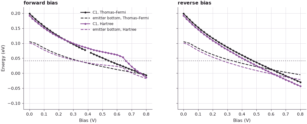
In reverse bias the Thomas–Fermi and Hartree traces almost coincide and both fall nearly linearly, at $-0.37$ eV/V; C1 passes the emitter Fermi level at 0.44–0.48 V. In forward bias the Hartree C1 starts with a similar slope ($-0.30$ eV/V against $-0.34$ eV/V below 0.3 V), but as the well fills it falls more and more slowly while the Thomas–Fermi C1 keeps falling: the Hartree C1 reaches the emitter Fermi level only at 0.66 V, 0.10 V later than the Thomas–Fermi one, and then drops abruptly as the well empties. The small step of the Thomas–Fermi trace near 0.4 V is an anticrossing of C1 with a state of the emitter notch. The emitter band bottom moves differently in the two models as well; the charge piled up in the well acts on the potential over a long range, including the emitter.

Slide 5: resonance energy traces and I–V in forward bias, Thomas–Fermi against Hartree — Slide 5. Forward bias in the lecture: (a) the central resonance C1 resists being pulled down and floats in the Fermi sea in the Hartree model; (b) the Hartree I–V is stretched out in voltage, quite linear, with a high valley current and a rapid turn-on after the valley.

The lecture also compares the forward and reverse band edges at the same bias: in forward bias the potential of the whole double barrier sits higher, because the accumulated charge counteracts the pull of the collector. With the emitter on the left in both cases, the same comparison here is:

Code31 lines · cell 21

v0 = 0.40
i0 = int(np.argmin(abs(V - v0)))
fig, ax = plt.subplots(figsize=(7, 4))
for name, color in (("forward", style.OPEN_NEMO), ("reverse", style.CONTEXT)):
    r = runs[name]
    ax.plot(
        r["d"].x, r["d"].band_edge + r["ha"]["potential"][i0], color=color, lw=1.8, label=f"{name} (Hartree)"
    )
    e, w = c1(r["d"], r["ha"]["potential"][i0], r["bl"], r["br"])
    ax.hlines(e, XB1 + r["bl"], XB1 + r["bl"] + 5, color=color, lw=2.5)
ax.set(
    xlabel="Position (nm)",
    ylabel="Energy (eV)",
    xlim=(55, 120),
    ylim=(-0.45, 0.45),
    title=f"Hartree conduction band at {v0:.2f} V",
)
ax.legend()

ef = traces["forward", "ha"]["c1"][:, 0]
er = traces["reverse", "ha"]["c1"][:, 0]
k0 = int(np.argmin(abs(VT - v0)))
v_match = np.interp(-ef[k0], -er, VT)  # reverse bias that puts C1 where forward C1 is at v0
print(
    f"C1 at {v0:.2f} V: forward {ef[k0] * 1e3:.1f} meV, reverse {er[k0] * 1e3:.1f} meV, "
    f"difference {(ef[k0] - er[k0]) * 1e3:.0f} meV"
)
print(
    f"reverse bias with the same C1 energy: {v_match:.2f} V, i.e. {v0 - v_match:.2f} V less; "
    f"lever (bias per C1 energy) {(v0 - v_match) / (ef[k0] - er[k0]):.1f} V/eV"
)

C1 at 0.40 V: forward 83.8 meV, reverse 50.5 meV, difference 33 meV
reverse bias with the same C1 energy: 0.28 V, i.e. 0.12 V less; lever (bias per C1 energy) 3.6 V/eV

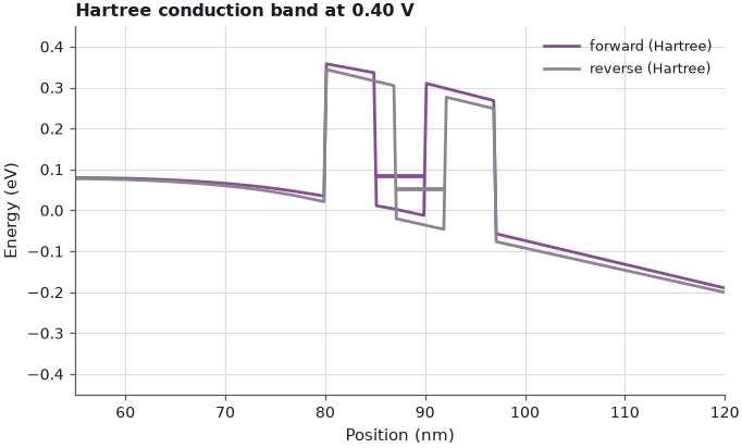
At 0.40 V the forward-bias C1 is 33 meV higher than the reverse-bias one, and the reverse structure needs 0.12 V less bias to put C1 at the same energy. The ratio, 3.6 V/eV, shows that only a fraction of the applied bias (about a quarter here) drops between the emitter and the well. The lecture quotes 100 meV for 0.24 V in its InGaAs device, a lever of 2.4 V/eV.

6. Current and sheet charge on a log scale#

The lecture's last calculation plots the current and the sheet charge in the well on a log scale in both directions. If $I = (e/\hbar)\Gamma_R n$ held with a fixed $\Gamma_R$, the two curves would have the same shape. The sheet density $n_s$ is the electron density integrated over the 5 nm well. The ratio $J/(e\, n_s)$ is an effective escape rate $1/\tau_\text{out}$; $\hbar/\tau_\text{out}$ is the corresponding energy, which can be compared with the zero-bias partial width of the collector barrier from section 1.

Code21 lines · cell 23

HBAR_EVS, Q = 6.582e-16, 1.602e-19
fig, axs = plt.subplots(2, 1, figsize=(7, 6.5), sharex=True)
for name, color in (("forward", style.OPEN_NEMO), ("reverse", style.CONTEXT)):
    r = runs[name]
    J = r["ha"]["current_density"]
    ns = r["ha"]["electron_density"][:, r["well"]].sum(axis=1) * 0.25e-7
    r["ns"] = ns
    axs[0].semilogy(V[1:], J[1:], color=color, lw=2, label=name)
    axs[1].semilogy(V, ns, color=color, lw=2, label=name)
    g_out = HBAR_EVS * J / (Q * np.maximum(ns, 1.0))
    g0 = G7 if name == "forward" else G5
    print(f"{name:8s} 0.0 V: n_s = {ns[0]:.2e} cm^-2 (equilibrium)")
    for v in (0.1, 0.3, 0.5, 0.7):
        i = int(np.argmin(abs(V - v)))
        print(
            f"{name:8s} {v:.1f} V: J = {J[i]:7.1f} A/cm^2, n_s = {ns[i]:.2e} cm^-2, "
            f"hbar/tau_out = {g_out[i] * 1e6:7.2f} ueV ({g_out[i] / g0:5.1f} x zero-bias Gamma_collector)"
        )
axs[0].set_ylabel("$J$ (A/cm$^2$)")
axs[1].set(xlabel="Bias (V)", ylabel="$n_s$ in the well (cm$^{-2}$)")
axs[0].legend();

forward  0.0 V: n_s = 2.12e+09 cm^-2 (equilibrium)
forward  0.1 V: J =     7.2 A/cm^2, n_s = 9.35e+09 cm^-2, hbar/tau_out =    3.16 ueV (  1.4 x zero-bias Gamma_collector)
forward  0.3 V: J =    73.7 A/cm^2, n_s = 5.77e+10 cm^-2, hbar/tau_out =    5.25 ueV (  2.3 x zero-bias Gamma_collector)
forward  0.5 V: J =   285.4 A/cm^2, n_s = 1.49e+11 cm^-2, hbar/tau_out =    7.86 ueV (  3.5 x zero-bias Gamma_collector)
forward  0.7 V: J =   440.9 A/cm^2, n_s = 1.25e+11 cm^-2, hbar/tau_out =   14.44 ueV (  6.5 x zero-bias Gamma_collector)
reverse  0.0 V: n_s = 2.12e+09 cm^-2 (equilibrium)
reverse  0.1 V: J =     5.5 A/cm^2, n_s = 6.64e+08 cm^-2, hbar/tau_out =   33.98 ueV (  0.7 x zero-bias Gamma_collector)
reverse  0.3 V: J =    43.4 A/cm^2, n_s = 2.06e+09 cm^-2, hbar/tau_out =   86.66 ueV (  1.9 x zero-bias Gamma_collector)
reverse  0.5 V: J =    36.9 A/cm^2, n_s = 4.96e+08 cm^-2, hbar/tau_out =  305.72 ueV (  6.6 x zero-bias Gamma_collector)
reverse  0.7 V: J =   100.0 A/cm^2, n_s = 4.41e+07 cm^-2, hbar/tau_out = 9311.88 ueV (199.7 x zero-bias Gamma_collector)

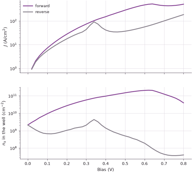
In forward bias the sheet density rises from its equilibrium value of $2.1\times10^{9}$ cm$^{-2}$ by two orders of magnitude up to the current peak, which is charge accumulation; in reverse bias it drops below the equilibrium value, apart from a bump at the peak, and falls to $4\times10^{7}$ cm$^{-2}$ at 0.7 V, which is charge depletion. The shapes of the current and charge curves are different, so the escape energy $\hbar/\tau_\text{out}$ changes with bias: in forward bias from 1.4 to 6.5 times the zero-bias partial width of the 7 nm barrier between 0.1 and 0.7 V, because the bias lowers the collector barrier as seen from the resonance. In reverse bias it grows by a factor of almost 300 between 0.1 and 0.7 V: once C1 is below the emitter band bottom the little current that flows is no longer carried by C1, and the ratio stops being a property of one level at all. The partial widths $\Gamma$ are strong functions of bias, which is why the lecture warns against using analytic formulas with fixed rates.

Slide 18: log current and sheet charge in the well in forward and reverse bias — Slide 18. (a) Current on a log scale and (b) sheet charge inside the RTD on a log scale in forward and reverse bias. Forward bias shows charge accumulation, reverse bias charge depletion; the different shapes of the current and charge curves show that $I = \Gamma_R n$ with a constant $\Gamma_R$ is not valid.

7. Experiment: systematically asymmetric devices#

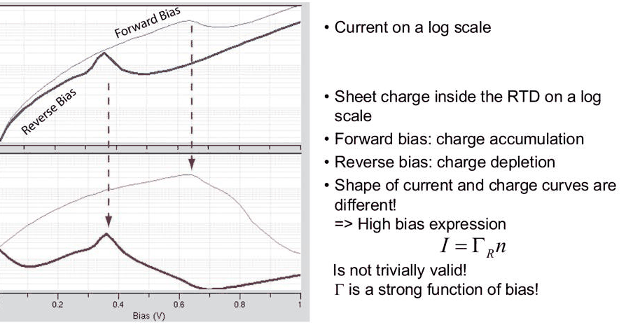
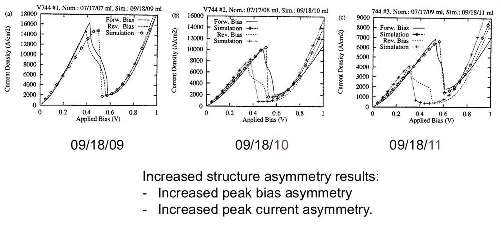
The asymmetric RTD was not an academic exercise. At the 1997 Device Research Conference (DRC 97) the NEMO team and Texas Instruments presented InGaAs/InAlAs RTDs with four nominally identical stacks, grown with systematic variations: spacer lengths of 20, 58, 117 and 200 Å around a 47/47/47 Å barrier/well/barrier, well widths of 29, 35 and 47 Å, and a set in which the collector barrier was 9, 10 and 11 monolayers thick. With increasing structural asymmetry the measured peak bias and peak current became increasingly different in forward and reverse bias, and NEMO reproduced the trends. The comparison was precise enough that the modelling could tell the growers that their layers were one or two monolayers off.

Slide 16: DRC 97 systematic test of asymmetric InGaAs/InAlAs RTDs — Slide 16. DRC 97: measured forward and reverse I–V curves and NEMO simulations of three devices whose collector barriers were grown 9, 10 and 11 monolayers thick. Increasing asymmetry increases the asymmetry of the peak bias and of the peak current.

The same experiment can be repeated numerically with the GaAs device: keep the 5 nm emitter barrier and change the collector barrier from 5 nm (symmetric) to 6 nm and 7 nm (the device above). Each Hartree I–V is computed in both directions on the same 0.02 V grid.

Code21 lines · cell 29

VE = V
fig, axs = plt.subplots(1, 3, figsize=(12, 3.6), sharey=True)
for ax, br in zip(axs, (5.0, 6.0, 7.0)):
    res = {}
    for name, (b1, b2) in (("forward", (5.0, br)), ("reverse", (br, 5.0))):
        if br == 7.0:
            J = runs[name]["ha"]["current_density"]
        else:
            J = nemo.hartree_iv(make_rtd(b1, b2), VE, T, quantum_charge=(-200, 200))["current_density"]
        k = first_peak(J)
        res[name] = (VE[k], J[k])
        ax.plot(VE, J, color=style.OPEN_NEMO if name == "forward" else style.CONTEXT, lw=2, label=name)
    (vf, jf), (vr, jr) = res["forward"], res["reverse"]
    print(
        f"collector barrier {br:.0f} nm: forward peak {jf:5.0f} A/cm^2 at {vf:.2f} V, reverse {jr:5.0f} "
        "A/cm^2 at "
        f"{vr:.2f} V; peak-bias ratio {vf / vr:.2f}, peak-current ratio {jf / jr:.1f}"
    )
    ax.set(xlabel="Bias (V)", title=f"5 nm / {br:.0f} nm barriers")
axs[0].set_ylabel("Current density (A/cm$^2$)")
axs[0].legend();

collector barrier 5 nm: forward peak  1893 A/cm^2 at 0.46 V, reverse  1893 A/cm^2 at 0.46 V; peak-bias ratio 1.00, peak-current ratio 1.0
collector barrier 6 nm: forward peak  1052 A/cm^2 at 0.54 V, reverse   437 A/cm^2 at 0.38 V; peak-bias ratio 1.42, peak-current ratio 2.4
collector barrier 7 nm: forward peak   521 A/cm^2 at 0.64 V, reverse    92 A/cm^2 at 0.34 V; peak-bias ratio 1.88, peak-current ratio 5.7

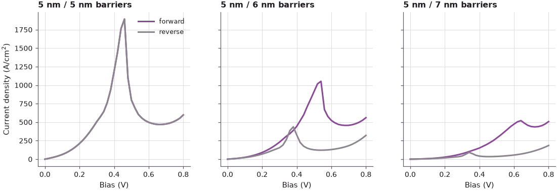
As in the DRC 97 devices, the asymmetry of both the peak bias and the peak current grows steadily with the thickness difference of the barriers. Since one nanometre is about three and a half monolayers of Al${0.3}$Ga${0.7}$As, a deviation of a single monolayer produces a measurable change, which is why the I–V curves could be used to check the growth.

Summary#

In a sequential picture with partial widths $\Gamma_L$ and $\Gamma_R$, the occupation of the well is $n = \Gamma_L/(\Gamma_L + \Gamma_R)$: close to 1 when the emitter barrier is thinner, close to 0 when it is thicker. Two nanometres of AlGaAs change $\Gamma$ by more than an order of magnitude.
Forward bias (5 nm emitter barrier): the well accumulates a sheet charge of order $10^{11}$ cm$^{-2}$, the electrostatic push-back keeps C1 up, and the Hartree I–V peak moves to a much higher voltage and current than the Thomas–Fermi one, with a higher valley current.
Reverse bias (7 nm emitter barrier): the well is nearly empty, resonances move linearly with bias, the Thomas–Fermi and Hartree models nearly agree, and the peak is at a smaller voltage with a much smaller current.
The current and the well charge have different bias dependences, so the effective tunneling rates are strong functions of bias; analytic formulas with constant rates must be used with caution.
Systematic barrier asymmetry produces a systematic forward/reverse asymmetry of the I–V, the effect used in the DRC 97 experiments to verify the modelling and the growth.

Exercises#

Use gamma_single to compute $\Gamma$ for barriers from 3 to 8 nm and fit $\ln\Gamma$ against the thickness. Compare the decay constant with $2\kappa$, $\kappa = \sqrt{2 m^* (E_b - E)}/\hbar$, at the C1 energy, and explain the difference.
Repeat the forward/reverse comparison with the Thomas–Fermi model only and with relaxation=None (ballistic). Which features of the asymmetry survive without the quantum charge in the loop?
Change the well of the 5 nm / 7 nm device to 4 nm and 6 nm. How do the forward Hartree peak voltage and the peak sheet density change, and why?
Make the emitter spacer 20 nm while keeping the collector spacer at 50 nm, with symmetric 5 nm barriers. Is the I–V asymmetric? Compare the size of the effect with that of a 1 nm barrier asymmetry.