Lecture 23.4

Theory of stress and strain — material response: elastic constants

In the lecture

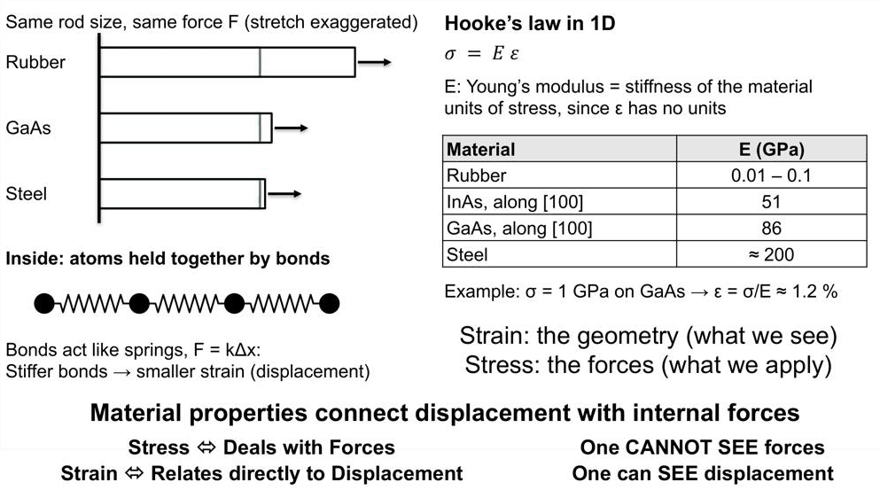
The same force stretches rubber, GaAs and steel by very different amounts: Hooke's law $\sigma = E\varepsilon$ with Young's modulus $E$, which comes from the stiffness of the bonds.
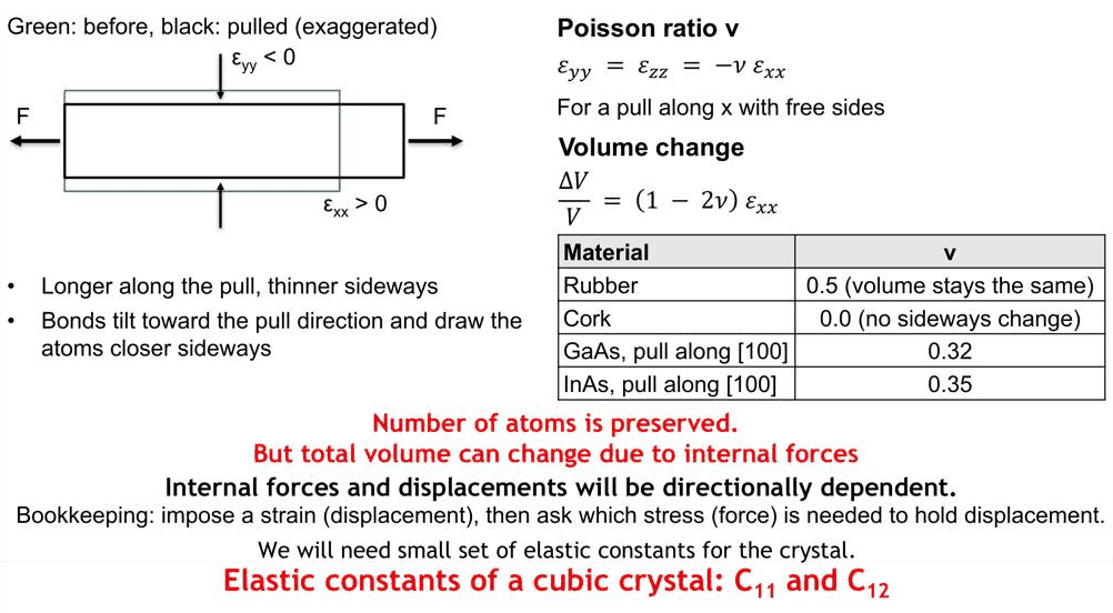
The Poisson effect: a bar pulled along $x$ gets thinner sideways, $\varepsilon_{yy} = \varepsilon_{zz} = -\nu\varepsilon_{xx}$, and its volume changes by $(1-2\nu)\varepsilon_{xx}$.
Hooke's law of a cubic crystal in Voigt notation: $C_{11}$ and $C_{12}$ for stretching, $C_{44}$ for shear; the signs of shear stress and why $\sigma_{xy} = \sigma_{yx}$.
Imposing stress and observing strain in three simple cases: the bulk modulus $B = (C_{11}+2C_{12})/3$, the Poisson ratio $\nu = C_{12}/(C_{11}+C_{12})$, and the thin-film ratio $\varepsilon_\perp/\varepsilon_\parallel = -2C_{12}/C_{11}$.
Where the constants come from: pressure with X-rays, pulled bars, strained layers and sound speeds, fitted together with more data than unknowns.

In this notebook

You build the 6 × 6 stiffness matrix of GaAs and InAs with elasticity.cubic_stiffness, compute Young's modulus along every direction (the crystal is not isotropic), pull a finite-element GaAs bar with free and with held sides to read off $E$, $\nu$, $C_{11}$ and $C_{12}$, check the torque balance behind $\sigma_{xy} = \sigma_{yx}$, solve the three stress cases of the lecture with the compliance matrix, compute the sound speeds of GaAs from its density, and fit $C_{11}$, $C_{12}$ and $C_{44}$ back from five noisy synthetic measurements.

Run the notebookEvery number and figure on this page comes from it. Change it, rerun it, take it further.

Download .ipynb View on GitHub

Run it on your own machine

The notebook needs open-nemo (Python ≥ 3.10 and a C++20 compiler; BLAS/LAPACK).

git clone https://github.com/denphi/open-nemo.git && cd open-nemo
python3 -m venv .venv && source .venv/bin/activate
pip install -e ".[notebooks]"
jupyter lab From_Atoms_to_Devices/09_stress_and_strain/23_4_material_response.ipynb

Code11 lines · cell 1

import numpy as np
import matplotlib.pyplot as plt
import opennemo as nemo
from opennemo.visualization import style
from scipy.optimize import least_squares
from opennemo.models import kp
from opennemo.models import mechanics as M
from opennemo.solvers import elasticity as E
from opennemo.solvers.poisson import Grid

style.use(notebook=True)

1. Same force, different stretch: Young's modulus#

Pull with the same force on rods of rubber, GaAs and steel of the same size: the rubber stretches a lot, the semiconductor much less and the steel even less. Inside, the atoms are held together by bonds that act like springs, $F = k\,\Delta x$; stiffer bonds give a smaller displacement, and so a smaller strain. For a rod this is Hooke's law,

\sigma = E\,\varepsilon ,

with Young's modulus $E$, the stiffness of the material. Because $\varepsilon$ has no units, $E$ has the units of stress. Strain is the geometry, what we see; stress is the force, what we apply. The material properties connect the two.

Slide 3: rubber, GaAs and steel under the same force, and Young's modulus — Slide 3. The same force stretches rods of rubber, GaAs and steel by different amounts (exaggerated). Young's moduli: rubber 0.01–0.1 GPa, InAs and GaAs along [100] 51 and 86 GPa, steel about 200 GPa. A stress of 1 GPa strains GaAs by about 1.2 %.

The values for the semiconductors carry a direction, [100], because a crystal is not isotropic: the bonds point along definite directions, and the stiffness depends on how the pull is oriented relative to them. In terms of the elastic constants introduced below, a cubic crystal has

\frac{1}{E(\mathbf{n})} = S_{11} - 2\left(S_{11} - S_{12} - \tfrac12 S_{44}\right) \left(n_x^2 n_y^2 + n_y^2 n_z^2 + n_z^2 n_x^2\right),

where $S = C^{-1}$ is the compliance matrix and $\mathbf{n}$ the unit vector along the pull. Along [100] this reduces to $E = (C_{11} - C_{12})(C_{11} + 2C_{12})/(C_{11} + C_{12})$. The measured constants are those of the Vurgaftman set in open-nemo (kp.material).

Code15 lines · cell 3

mats = {name: kp.material(name) for name in ("GaAs", "InAs")}
C = {name: E.cubic_stiffness(m.c11, m.c12, m.c44) for name, m in mats.items()}   # 6x6, GPa
print("GaAs stiffness matrix C (GPa), Voigt order xx, yy, zz, yz, xz, xy:\n", np.round(C["GaAs"], 1))

def young(Cm, n):
    Sm = np.linalg.inv(Cm)
    n = np.asarray(n, float) / np.linalg.norm(n)
    q = n[0]**2 * n[1]**2 + n[1]**2 * n[2]**2 + n[2]**2 * n[0]**2
    return 1 / (Sm[0, 0] - 2 * (Sm[0, 0] - Sm[0, 1] - 0.5 * Sm[3, 3]) * q)

for name, m in mats.items():
    e100 = (m.c11 - m.c12) * (m.c11 + 2 * m.c12) / (m.c11 + m.c12)
    print(f"{name}: E[100] = {young(C[name], [1, 0, 0]):.1f} GPa (formula {e100:.1f}),  "
          f"E[110] = {young(C[name], [1, 1, 0]):.1f},  E[111] = {young(C[name], [1, 1, 1]):.1f} GPa;  "
          f"strain at 1 GPa along [100]: {100 / young(C[name], [1, 0, 0]):.2f} %")

GaAs stiffness matrix C (GPa), Voigt order xx, yy, zz, yz, xz, xy:
 [[122.1  56.6  56.6   0.    0.    0. ]
 [ 56.6 122.1  56.6   0.    0.    0. ]
 [ 56.6  56.6 122.1   0.    0.    0. ]
 [  0.    0.    0.   60.    0.    0. ]
 [  0.    0.    0.    0.   60.    0. ]
 [  0.    0.    0.    0.    0.   60. ]]
GaAs: E[100] = 86.2 GPa (formula 86.2),  E[110] = 123.0,  E[111] = 143.4 GPa;  strain at 1 GPa along [100]: 1.16 %
InAs: E[100] = 51.4 GPa (formula 51.4),  E[110] = 79.3,  E[111] = 96.7 GPa;  strain at 1 GPa along [100]: 1.94 %

Code20 lines · cell 4

phi = np.linspace(0, 2 * np.pi, 361)
fig, (ax1, ax2) = plt.subplots(1, 2, figsize=(10, 4.2), gridspec_kw={"width_ratios": [1.2, 1]})
ref = {"rubber": (0.01, 0.1), "steel": (200, 200)}
names = ["rubber", "InAs [100]", "GaAs [100]", "GaAs [111]", "steel"]
vals = [0.05, young(C["InAs"], [1, 0, 0]), young(C["GaAs"], [1, 0, 0]), young(C["GaAs"], [1, 1, 1]), 200]
ax1.barh(names, vals, color=[style.CONTEXT, style.OPEN_NEMO, style.OPEN_NEMO, style.OPEN_NEMO, style.CONTEXT])
ax1.errorbar([0.05], [0], xerr=[[0.04], [0.05]], fmt="none", color="k", capsize=3)
ax1.set_xscale("log")
ax1.set_xlabel("Young's modulus E (GPa)")
ax1.set_title("Same force, different stretch")
for name, col in (("GaAs", style.OPEN_NEMO), ("InAs", style.REFERENCE)):
    Ephi = np.array([young(C[name], [np.cos(p), np.sin(p), 0]) for p in phi])
    ax2.plot(Ephi * np.cos(phi), Ephi * np.sin(phi), color=col, label=name)
ax2.set_aspect("equal")
ax2.set_xlabel("E along x (GPa)")
ax2.set_ylabel("E along y (GPa)")
ax2.set_title("E(n) for pulls in the (001) plane")
ax2.legend(fontsize=8)
plt.tight_layout()
plt.show()

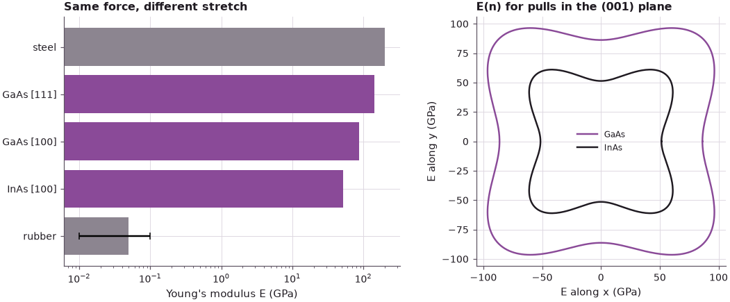
Figure computed by the notebook with open-nemo

GaAs has $E = 86.2$ GPa along [100] and 123.0 GPa along [110]; InAs 51.4 GPa along [100]. A stress of 1 GPa along [100] stretches GaAs by 1.16 %, the slide's 1.2 % (and InAs by 1.94 %). The polar plot shows the anisotropy: GaAs is stiffest along the face diagonals in the (001) plane (and stiffer still along [111], 143.4 GPa), where a pull bends bonds less and stretches them more.

2. Pull in one direction, shrink in the others: the Poisson effect#

A bar pulled along $x$ gets longer along the pull and thinner sideways. The bonds tilt towards the pull and draw the atoms closer together sideways. For a pull along $x$ with free sides the Poisson ratio $\nu$ describes the sideways strain,

\varepsilon_{yy} = \varepsilon_{zz} = -\nu\,\varepsilon_{xx}, \qquad \frac{\Delta V}{V} = (1 - 2\nu)\,\varepsilon_{xx} .

Rubber has $\nu \approx 0.5$: its volume stays the same. Cork has $\nu \approx 0$: it does not widen when squeezed, which is why it can be pushed into a bottle. GaAs and InAs pulled along [100] have 0.32 and 0.35. The number of atoms is fixed, but the volume can change under internal forces, and a deformed solid stores energy. Because these responses depend on direction, a small set of elastic constants is needed for the bookkeeping.

Slide 4: the Poisson effect — Slide 4. A bar pulled along $x$ (green before, black after, exaggerated) becomes longer and thinner; the table lists Poisson ratios from rubber (0.5) to cork (0.0).

Lecture 23.3 pulled a finite-element GaAs rod with free sides. The same experiment gives both $E$ and $\nu$, and a second run with the sides held (periodic in $y$ and $z$, so their size cannot change) gives the bookkeeping constants directly: then $\sigma_{xx} = C_{11}\varepsilon_{xx}$ and the force needed to hold the sides is $\sigma_{yy} = \sigma_{zz} = C_{12}\varepsilon_{xx}$.

Code20 lines · cell 6

def pull(Cm, held_sides, length=10.0, width=2.0, stretch=0.01):
    g = Grid(np.linspace(0, length, 21), np.linspace(0, width, 5), np.linspace(0, width, 5))
    el = E.Elasticity(g, Cm, periodic=(False, held_sides, held_sides))
    X = g.nodes
    el.fix(np.isclose(X[:, 0], 0), (0,), 0.0)
    el.fix(np.isclose(X[:, 0], length), (0,), stretch)
    el.fix(np.flatnonzero(np.all(np.isclose(X, 0), axis=1)), (1, 2), 0.0)
    el.fix(np.flatnonzero(np.all(np.isclose(X, [0, width, 0]), axis=1)), (2,), 0.0)
    r = el.solve()
    return r.strain.mean(axis=0), r.stress.mean(axis=0)

for name, m in mats.items():
    eps, sig = pull(C[name], held_sides=False)
    nu, Ey = -eps[1, 1] / eps[0, 0], sig[0, 0] / eps[0, 0]
    print(f"{name}, free sides: E = {Ey:.1f} GPa, ν = {nu:.4f} "
          f"(C12/(C11+C12) = {m.c12 / (m.c11 + m.c12):.4f}), "
          f"ΔV/V = {100 * np.trace(eps):.4f} % = (1−2ν) ε_xx")
    eps, sig = pull(C[name], held_sides=True)
    print(f"{name}, held sides: σ_xx/ε_xx = {sig[0, 0] / eps[0, 0]:.1f} GPa (C11 = {m.c11:.1f}),  "
          f"σ_yy/ε_xx = {sig[1, 1] / eps[0, 0]:.1f} GPa (C12 = {m.c12:.1f})")

GaAs, free sides: E = 86.2 GPa, ν = 0.3167 (C12/(C11+C12) = 0.3167), ΔV/V = 0.0367 % = (1−2ν) ε_xx
GaAs, held sides: σ_xx/ε_xx = 122.1 GPa (C11 = 122.1),  σ_yy/ε_xx = 56.6 GPa (C12 = 56.6)
InAs, free sides: E = 51.4 GPa, ν = 0.3521 (C12/(C11+C12) = 0.3521), ΔV/V = 0.0296 % = (1−2ν) ε_xx
InAs, held sides: σ_xx/ε_xx = 83.3 GPa (C11 = 83.3),  σ_yy/ε_xx = 45.3 GPa (C12 = 45.3)

With free sides the bar gives $E = 86.2$ GPa and $\nu = 0.3167$ for GaAs (51.4 GPa and 0.3521 for InAs), exactly the closed-form values; a 0.1 % stretch increases the volume by $(1-2\nu)\,0.1\,\% = 0.0367\,\%$. With the sides held, the stress along the pull is $C_{11}\varepsilon_{xx}$ and a sideways stress $C_{12}\varepsilon_{xx}$ is needed to keep the bar from narrowing: $C_{12} > 0$ means the cell wants to shrink sideways, the Poisson effect again.

3. Hooke's law of a cubic crystal: $C_{11}$, $C_{12}$ and $C_{44}$#

Imposing one stretch at a time and superposing (the theory is linear) gives

\sigma_{xx} = C_{11}\varepsilon_{xx} + C_{12}(\varepsilon_{yy} + \varepsilon_{zz}),

and the same for $y$ and $z$; cubic symmetry makes $x$, $y$ and $z$ equivalent, so two constants serve every axis. Shear needs care with signs. On a small square, the stress times the outward normal of a face is the force per area on it, the traction $t_i = \sum_j \sigma_{ij} n_j$. Opposite faces have opposite normals, so their forces are opposite and the net force vanishes. The top/bottom pair, however, turns the square one way and the side pair the other, and the square stays at rest only if the two torques cancel, which requires $\sigma_{xy} = \sigma_{yx}$.

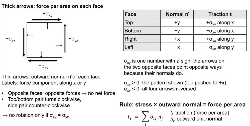
Slide 6: signs of the shear stresses on a small square — Slide 6. Thick arrows: force per area on each face; thin arrows: outward normals. The top and bottom forces turn the square clockwise, the side forces counter-clockwise; there is no rotation only if $\sigma_{xy} = \sigma_{yx}$.

The torque balance can be checked by summing $\mathbf{r} \times \mathbf{t}\,A$ over the four faces of a unit square:

Code16 lines · cell 8

faces = {"top": [0, 1], "bottom": [0, -1], "right": [1, 0], "left": [-1, 0]}       # outward normals

def net_torque(s_xy, s_yx, side=1.0):
    sig = np.array([[0.0, s_xy], [s_yx, 0.0]])        # σ_ij: force along i on the face with normal j
    force, torque = np.zeros(2), 0.0
    for n in faces.values():
        n = np.array(n, float)
        t = sig @ n                                    # traction on that face (GPa)
        r = 0.5 * side * n                             # face centre
        force += t * side
        torque += (r[0] * t[1] - r[1] * t[0]) * side
    return force, torque

for s_xy, s_yx in ((1.0, 1.0), (1.0, 0.5)):
    f, tq = net_torque(s_xy, s_yx)
    print(f"σ_xy = {s_xy}, σ_yx = {s_yx} GPa: net force {f} , net torque {tq:+.2f} (GPa · area · length)")

σ_xy = 1.0, σ_yx = 1.0 GPa: net force [0. 0.] , net torque +0.00 (GPa · area · length)
σ_xy = 1.0, σ_yx = 0.5 GPa: net force [0. 0.] , net torque -0.50 (GPa · area · length)

With $\sigma_{xy} = \sigma_{yx}$ both the net force and the net torque vanish; with $\sigma_{yx} = \sigma_{xy}/2$ a torque of magnitude 0.5 (in units of GPa times area times length) is left over and the square would spin. Shear is described by a third constant. A shear strain changes angles, not lengths: the side edges tilt by $\theta \approx 2\varepsilon_{xy}$ (Lecture 23.2), and

\sigma_{xy} = 2C_{44}\,\varepsilon_{xy},

with the same $C_{44}$ for $yz$ and $xz$. In a cubic crystal stretching along the cube axes and shear are independent. Altogether, in Voigt's notation (xx → 1, yy → 2, zz → 3, yz → 4, xz → 5, xy → 6; W. Voigt, Lehrbuch der Kristallphysik, 1910),

\begin{pmatrix}\sigma_{xx}\\ \sigma_{yy}\\ \sigma_{zz}\\ \sigma_{yz}\\ \sigma_{xz}\\ \sigma_{xy}\end{pmatrix} = \begin{pmatrix} C_{11} & C_{12} & C_{12} & 0 & 0 & 0\\ C_{12} & C_{11} & C_{12} & 0 & 0 & 0\\ C_{12} & C_{12} & C_{11} & 0 & 0 & 0\\ 0 & 0 & 0 & C_{44} & 0 & 0\\ 0 & 0 & 0 & 0 & C_{44} & 0\\ 0 & 0 & 0 & 0 & 0 & C_{44} \end{pmatrix} \begin{pmatrix}\varepsilon_{xx}\\ \varepsilon_{yy}\\ \varepsilon_{zz}\\ 2\varepsilon_{yz}\\ 2\varepsilon_{xz}\\ 2\varepsilon_{xy}\end{pmatrix},

the matrix printed in Section 1. The factor 2 on the shear strains is the engineering shear angle. For GaAs $C_{11} = 122.1$, $C_{12} = 56.6$ and $C_{44} = 60.0$ GPa; for InAs 83.3, 45.3 and 39.6 GPa. The general form $\sigma_{ij} = \sum_{kl} C_{ijkl}\varepsilon_{kl}$ applies to any crystal; cubic symmetry leaves only these three independent numbers.

4. Imposing stress, observing strain: three simple cases#

So far a strain was imposed and the stress needed to hold it was computed. Experiments work the other way: they apply a known stress (a measurable force) and observe the strain. That means inverting Hooke's law, $\boldsymbol{\varepsilon} = S\boldsymbol{\sigma}$ with $S = C^{-1}$. Three cases are simple:

(a) pressure from all sides, $\sigma_{ij} = -p\,\delta_{ij}$: $-p = B\,\mathrm{Tr}\,\boldsymbol{\varepsilon}$ with the bulk modulus $B = (C_{11} + 2C_{12})/3$;
(b) pull along $x$ with free sides: $\varepsilon_{yy} = \varepsilon_{zz} = -\nu\,\varepsilon_{xx}$ with $\nu = C_{12}/(C_{11} + C_{12})$;
(c) squeeze in $x$ and $y$ with the top free, $\sigma_{zz} = C_{11}\varepsilon_{zz} + 2C_{12}\varepsilon_{xx} = 0$: $\varepsilon_\perp/\varepsilon_\parallel = -2C_{12}/C_{11}$. This is a thin film on a thick substrate: the substrate imposes the in-plane size, the top surface is free, and a film squeezed in-plane grows taller out of plane (Lecture 23.5).

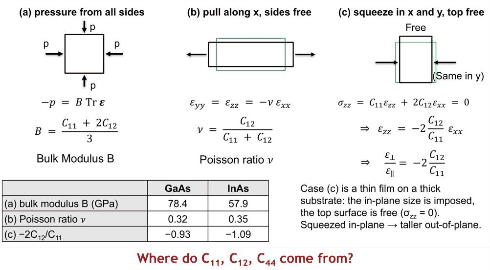
Slide 9: three ways to impose stress and observe strain — Slide 9. (a) Hydrostatic pressure gives the bulk modulus $B$, (b) a pull with free sides the Poisson ratio $\nu$, (c) an in-plane squeeze with a free top the ratio $-2C_{12}/C_{11}$. GaAs: 78.4 GPa, 0.32, −0.93; InAs: 57.9 GPa, 0.35, −1.09.

The cell below solves the three cases with the full compliance matrix (case (c) by imposing $\sigma_{zz} = 0$ with the in-plane strain given) and compares with the closed forms.

Code14 lines · cell 10

v2t = E.voigt_to_strain
print(f"{'':6s}{'B (GPa)':>18s}{'ν':>18s}{'ε⊥/ε∥':>20s}")
for name, m in mats.items():
    Sm = np.linalg.inv(C[name])
    p = 1.0                                                      # (a) 1 GPa of pressure
    eps_a = Sm @ np.array([-p, -p, -p, 0, 0, 0])
    B_num = -p / eps_a[:3].sum()
    eps_b = Sm @ np.array([1.0, 0, 0, 0, 0, 0])                  # (b) 1 GPa pull along x
    nu_num = -eps_b[1] / eps_b[0]
    e_par = -0.01                                                # (c) ε_xx = ε_yy given, σ_zz = 0
    e_perp = -(C[name][2, 0] + C[name][2, 1]) * e_par / C[name][2, 2]
    print(f"{name:6s}{B_num:9.1f} ({(m.c11 + 2 * m.c12) / 3:5.1f})"
          f"{nu_num:10.4f} ({m.c12 / (m.c11 + m.c12):.4f})"
          f"{e_perp / e_par:11.4f} ({-2 * m.c12 / m.c11:.4f})")

                 B (GPa)                 ν               ε⊥/ε∥
GaAs       78.4 ( 78.4)    0.3167 (0.3167)    -0.9271 (-0.9271)
InAs       57.9 ( 57.9)    0.3521 (0.3521)    -1.0868 (-1.0868)

The numerical inversions reproduce the closed forms (in brackets): $B$ = 78.4 and 57.9 GPa, $\nu$ = 0.3167 and 0.3521, $\varepsilon_\perp/\varepsilon_\parallel$ = −0.9271 and −1.0868 for GaAs and InAs, the slide's table. The last ratio is the one that will matter most: an InAs film squeezed in-plane by 1 % grows by 1.09 % out of plane, a GaAs film by 0.93 %.

5. Where do $C_{11}$, $C_{12}$ and $C_{44}$ come from?#

No single experiment measures the elastic constants. Several measure easy combinations of them:

Experiment	Measured quantity	Relation to C
hydrostatic pressure + X-ray lattice constant	bulk modulus $B$	$B = (C_{11} + 2C_{12})/3$
pull a bar along [100], strain gauges	Poisson ratio $\nu$	$\nu = C_{12}/(C_{11} + C_{12})$
X-ray diffraction of a strained (001) layer	$\varepsilon_\perp/\varepsilon_\parallel$	$-2C_{12}/C_{11}$
longitudinal sound wave along [100]	speed $v_L$	$\rho v_L^2 = C_{11}$
transverse sound wave along [100]	speed $v_T$	$\rho v_T^2 = C_{44}$

Here $\rho$ is the mass density; the sound speeds come from ultrasound or Brillouin scattering. The density follows from the crystal itself: a zincblende cubic cell of edge $a$ holds four Ga and four As atoms.

Code7 lines · cell 12

amu = 1.66053907e-27                                             # kg
gaas = mats["GaAs"]
a_m = gaas.lattice_constant * 1e-9
rho = 4 * (M.ATOMIC_MASS["Ga"] + M.ATOMIC_MASS["As"]) * amu / a_m**3                     # kg/m^3
vL, vT = np.sqrt(gaas.c11 * 1e9 / rho), np.sqrt(gaas.c44 * 1e9 / rho)
print(f"GaAs: a = {10 * gaas.lattice_constant:.4f} Å, ρ = {rho / 1000:.3f} g/cm³, "
      f"v_L = {vL / 1000:.2f} km/s, v_T = {vT / 1000:.2f} km/s")

GaAs: a = 5.6532 Å, ρ = 5.318 g/cm³, v_L = 4.79 km/s, v_T = 3.36 km/s

The density is 5.318 g/cm³ and the longitudinal sound speed along [100] is 4.79 km/s, the slide's 4.8 km/s; the transverse wave is slower, 3.36 km/s, because $C_{44} < C_{11}$.

Five measurements for three unknowns: the constants are fitted, and the excess data is a consistency check, because each experiment has its own error. The cell below plays this game. It generates the five "measured" quantities from the GaAs constants, adds 1 % random error to each, and fits $C_{11}$, $C_{12}$ and $C_{44}$ to them by least squares (each residual normalised by its 1 % uncertainty).

Code16 lines · cell 14

def observables(c):
    c11, c12, c44 = c
    return np.array([(c11 + 2 * c12) / 3, c12 / (c11 + c12), -2 * c12 / c11,
                     np.sqrt(c11 * 1e9 / rho), np.sqrt(c44 * 1e9 / rho)])

labels = ["B (GPa)", "ν", "ε⊥/ε∥", "v_L (m/s)", "v_T (m/s)"]
true = np.array([gaas.c11, gaas.c12, gaas.c44])
rng = np.random.default_rng(7)
meas = observables(true) * (1 + 0.01 * rng.standard_normal(5))
fit = least_squares(lambda c: (observables(c) - meas) / (0.01 * np.abs(meas)), x0=[100.0, 50.0, 50.0])
cov = np.linalg.inv(fit.jac.T @ fit.jac)
for lab, mv, fv in zip(labels, meas, observables(fit.x)):
    print(f"{lab:10s} measured {mv:10.4f}   fitted {fv:10.4f}")
for name, t, f, s in zip(("C11", "C12", "C44"), true, fit.x, np.sqrt(np.diag(cov))):
    print(f"{name}: fitted {f:6.1f} ± {s:4.1f} GPa   (true {t:.1f})")
print(f"χ² = {2 * fit.cost:.2f} for 5 − 3 = 2 degrees of freedom")

B (GPa)    measured    78.4343   fitted    78.1554
ν          measured     0.3177   fitted     0.3169
ε⊥/ε∥      measured    -0.9246   fitted    -0.9277
v_L (m/s)  measured  4749.1331   fitted  4782.5482
v_T (m/s)  measured  3343.7834   fitted  3343.7834
C11: fitted  121.6 ±  1.2 GPa   (true 122.1)
C12: fitted   56.4 ±  0.6 GPa   (true 56.6)
C44: fitted   59.5 ±  1.2 GPa   (true 60.0)
χ² = 0.80 for 5 − 3 = 2 degrees of freedom

The fit returns $C_{11} = 121.6 \pm 1.2$, $C_{12} = 56.4 \pm 0.6$ and $C_{44} = 59.5 \pm 1.2$ GPa against the true 122.1, 56.6 and 60.0, and a $\chi^2$ of 0.80 for two degrees of freedom: the five measurements are consistent with one set of three constants. Had one experiment a systematic error, $\chi^2$ would be large and the constants biased, which is exactly why several independent measurements are made. Note also that $C_{44}$ rests on a single observable, the transverse sound speed.

An atomistic model must reproduce these same constants. Lecture 23.1 computed them with the Keating valence force field and found $C_{11}$ and $C_{12}$ close but $C_{44}$ too low; the elastic constants are the bridge that lets continuum and atomistic models be compared.

Summary#

Elastic constants link strain (geometry, visible) and stress (forces, invisible). In one dimension $\sigma = E\varepsilon$; GaAs has $E = 86.2$ GPa along [100] (1 GPa → 1.16 % strain), 143.4 GPa along [111]: a crystal is anisotropic.
A pulled bar narrows: $\nu = C_{12}/(C_{11} + C_{12})$ = 0.3167 for GaAs, 0.3521 for InAs; its volume changes by $(1 - 2\nu)\varepsilon_{xx}$.
A cubic crystal needs three constants: $C_{11}$ and $C_{12}$ for stretching, $C_{44}$ for shear, arranged in Voigt's 6 × 6 matrix; $\sigma_{xy} = \sigma_{yx}$ because the torques must cancel.
Imposed stresses give $B = (C_{11} + 2C_{12})/3$ (78.4 and 57.9 GPa), $\nu$, and the thin-film ratio $\varepsilon_\perp/\varepsilon_\parallel = -2C_{12}/C_{11}$ (−0.93 and −1.09).
The constants are fitted to several measurements, including sound speeds ($v_L = 4.79$ km/s in GaAs); more data than unknowns is a consistency check.

Exercises#

Plot $E(\mathbf{n})$ of GaAs in the (1$\bar{1}$0) plane, which contains [001], [111] and [110]. Where is it largest? Compute the Zener anisotropy ratio $2C_{44}/(C_{11} - C_{12})$ of GaAs and InAs; an isotropic material has 1.
Repeat the fit of Section 5 with a 5 % systematic error on the bulk modulus only. How do $\chi^2$ and the fitted constants change? Which constant is affected most?
Compute $v_L$ and $v_T$ along [100] for InAs (density from M.ATOMIC_MASS["In"]) and compare with GaAs.
Pull the finite-element bar of Section 2 along [110] instead of [100] by rotating the stiffness matrix (or by computing $E$[110] with young) and compare $E$.

Experiment	Measured quantity	Relation to C
hydrostatic pressure + X-ray lattice constant	bulk modulus \(B\)	\(B = (C_{11} + 2C_{12})/3\)
pull a bar along [100], strain gauges	Poisson ratio \(\nu\)	\(\nu = C_{12}/(C_{11} + C_{12})\)
X-ray diffraction of a strained (001) layer	\(\varepsilon_\perp/\varepsilon_\parallel\)	\(-2C_{12}/C_{11}\)
longitudinal sound wave along [100]	speed \(v_L\)	\(\rho v_L^2 = C_{11}\)
transverse sound wave along [100]	speed \(v_T\)	\(\rho v_T^2 = C_{44}\)