Course/03 · Tunneling and band structure

ECE 606 Lecture 7.1

Band structure in a periodic potential — problem formulation

In the lecture

from $N$ barriers to infinitely many: when the structure is long, the electron cannot tell it from a periodic one
the smallest unit cell, a well of width $a$ and a barrier of width $b$, period $L = a + b$
Bloch's theorem $\psi(x + L) = e^{ikL}\psi(x)$, and a ring of $N$ cells that makes the allowed wave numbers $k = 2\pi n/(NL)$ with $-\pi/L \le k < \pi/L$
the five steps of the analytical solution adapted to a periodic system: four boundary conditions in one cell, one of them carrying the phase $e^{ikL}$
the determinant condition $\cos kL = f(E/U_0)$, the Kronig–Penney equation

In this notebook

builds a ring of identical cells with open-nemo's discretized Hamiltonian and shows that its eigenvalues are those of single-cell Bloch problems at $k = 2\pi n/(NL)$, sets up the 4×4 boundary-condition matrix of the lecture and checks that its determinant is the Kronig–Penney function, compares the analytical bands with nemo.lead_bands, and explores the complex wave numbers in the gaps with nemo.complex_bands.

Run the notebookEvery number and figure on this page comes from it. Change it, rerun it, take it further.

Download .ipynb View on GitHub

Run it on your own machine

The notebook needs open-nemo (Python ≥ 3.10 and a C++20 compiler; BLAS/LAPACK).

git clone https://github.com/denphi/open-nemo.git && cd open-nemo
python3 -m venv .venv && source .venv/bin/activate
pip install -e ".[notebooks]"
jupyter lab From_Atoms_to_Devices/03_tunneling_and_bandstructure/07_1_bandstructure_problem_formulation.ipynb

Code8 lines · cell 1

import numpy as np
import matplotlib.pyplot as plt
import opennemo as nemo
from opennemo.visualization import style

style.use(notebook=True)
H2M0 = nemo.core.units.HBAR2_2M0          # ħ²/2m₀ = 0.0381 eV nm²
EM = nemo.structures.materials.EffectiveMassMaterial

1. From many barriers to a periodic potential#

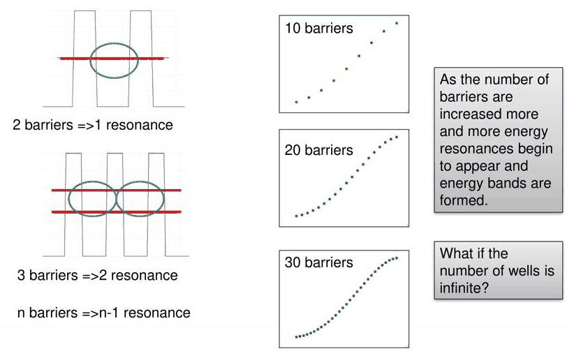
In Lecture 6.4 a stack of $N$ barriers produced $N - 1$ transmission resonances that lined up into bands as $N$ grew. A real solid has of the order of $10^{23}$ atoms; an explicit calculation with two unknown coefficients per region is out of the question. The way out is to treat the structure as infinitely repeated. Far from its ends an electron cannot distinguish a long stack from a periodic potential $U(x + L) = U(x)$, and periodicity can be exploited analytically.

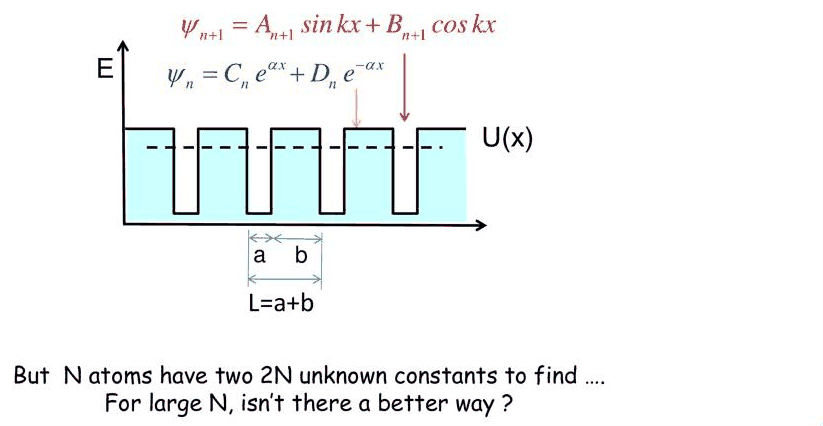
Slide 3: transmission through repeated wells — Slide 3: $n$ barriers give $n - 1$ resonances; with 10, 20 and 30 barriers the resonances fill energy bands. What if the number of wells is infinite?

The computational unit is the smallest repeating cell. As in the lecture it contains one well of width $a$, where the potential is 0, and one barrier of width $b$ and height $U_0$: period $L = a + b$. The numbers used throughout are those of the lecture's GaAs example in Lecture 7.2: $a = 6$ nm, $b = 2$ nm, $U_0 = 0.4$ eV, effective mass $m = 0.067\,m_0$ in both materials.

Slide 10: the unit cell and the ansatz — Slide 10: sinusoids in the well, exponentials in the barrier. $N$ cells would have $2N$ unknown constants; for large $N$ a better way is needed.

Code11 lines · cell 3

M, A, B, U0, DX = 0.067, 6.0, 2.0, 0.4, 0.05
L = A + B

cell = nemo.Heterostructure1D(
    [nemo.Layer(EM("GaAs", M, 12.9), A), nemo.Layer(EM("barrier", M, 12.9, conduction_band_edge=U0), B)],
    spacing=DX,
)
h = cell.hamiltonian.sparse.dense().real  # one cell, end sites already carry 2t0 on the diagonal
V = np.zeros_like(h)
V[-1, 0] = -H2M0 / (M * DX**2)  # bond from the last site of a cell to the first of the next
print(f"one cell: {cell.num_sites} sites of {DX} nm, period L = {L} nm, t0 = {-V[-1, 0]:.2f} eV")

one cell: 160 sites of 0.05 nm, period L = 8.0 nm, t0 = 227.46 eV

2. Bloch's theorem and the ring of N cells#

If $U$ is periodic, $|\psi|^2$ must be periodic too: the electron density in one cell is the same as in the next. The wave function itself may differ by a phase,

\psi(x + L) = e^{ikL}\,\psi(x),

Bloch's theorem, after the Swiss-American physicist Felix Bloch. The $k$ here labels the phase per cell; it is not the local wave number $\sqrt{2mE}/\hbar$ of the earlier lectures. Across $N$ cells the phase accumulates to $e^{ikNL}$. Klimeck's thought experiment ("Gedanken experiment") closes the chain of $N$ cells into a ring, so that cell $N + 1$ is cell 1 again. Then $e^{ikNL} = 1$, and

k = \frac{2\pi n}{NL}, \qquad n = -\frac N2, \dots, \frac N2 - 1, \qquad -\frac{\pi}{L} \le k < \frac{\pi}{L}.

$N$ is arbitrary but fixed; it sets how densely $k$ is sampled, not which energies are possible.

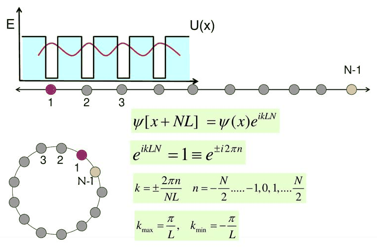
Slide 14: the periodic boundary condition — Slide 14: the ring of $N$ cells, $e^{ikLN} = 1$, and the range $k_\mathrm{min} = -\pi/L$, $k_\mathrm{max} = \pi/L$.

The theorem can be tested directly. The ring Hamiltonian of $N$ cells is block-circulant: the cell matrix $h$ on the diagonal and the inter-cell bond $V$ between neighbours, including the bond from cell $N$ back to cell 1. Its eigenvalues are compared with those of the one-cell Bloch Hamiltonian $H(k) = h + Ve^{ikL} + V^Te^{-ikL}$ at the $N$ allowed values of $k$.

Code21 lines · cell 5

N = 8
S = np.roll(np.eye(N), 1, axis=1)  # S[j, j+1] = 1, and S[N-1, 0] = 1 closes the ring
H_ring = np.kron(np.eye(N), h) + np.kron(S, V) + np.kron(S.T, V.T)
E_ring = np.linalg.eigvalsh(H_ring)


def bloch_h(k):
    return h + V * np.exp(1j * k * L) + V.T * np.exp(-1j * k * L)


ks = 2 * np.pi * np.arange(-N // 2, N // 2) / (N * L)
E_bloch = np.array([np.linalg.eigvalsh(bloch_h(k))[:3] for k in ks])  # (N k values, 3 bands)
lowest = np.sort(E_bloch.ravel())[: 2 * N]
print(f"ring of {N} cells: {H_ring.shape[0]} sites; one cell: {h.shape[0]} sites")
print(
    f"largest difference between the lowest {2 * N} ring eigenvalues and the Bloch eigenvalues: "
    f"{np.abs(E_ring[: 2 * N] - lowest).max():.1e} eV"
)
print("  n    k (1/nm)   band 1 (eV)   band 2 (eV)")
for n, k, e in zip(range(-N // 2, N // 2), ks, E_bloch):
    print(f" {n:3d}   {k:7.4f}     {e[0]:.5f}      {e[1]:.5f}")

ring of 8 cells: 1280 sites; one cell: 160 sites
largest difference between the lowest 16 ring eigenvalues and the Bloch eigenvalues: 6.7e-13 eV
  n    k (1/nm)   band 1 (eV)   band 2 (eV)
  -4   -0.3927     0.09611      0.23989
  -3   -0.2945     0.08922      0.25646
  -2   -0.1963     0.07595      0.29789
  -1   -0.0982     0.06547      0.35001
   0    0.0000     0.06166      0.38225
   1    0.0982     0.06547      0.35001
   2    0.1963     0.07595      0.29789
   3    0.2945     0.08922      0.25646

The $8 \times 160 = 1280$-site ring and eight 160-site Bloch problems give the same eigenvalues to round-off. Every band contains exactly $N = 8$ states, one per allowed $k$; states at $+k$ and $-k$ are degenerate, and the lowest band runs from 0.0617 eV at $k = 0$ to 0.0961 eV at the zone boundary $k = -\pi/L$. This is the computational gain of Bloch's theorem: an $N$-cell problem becomes $N$ one-cell problems, and $N$ can then be made as large as desired at no extra cost per state.

3. The boundary conditions in one cell#

The lecture now follows the five steps of the analytical solution, with two changes. The edge conditions are replaced by Bloch's theorem, and the interface conditions are written for one cell. Put the barrier at $-b < x < 0$ and the well at $0 < x < a$, with

\psi_a = A_a\sin\alpha x + B_a\cos\alpha x, \qquad \psi_b = A_b\sin\beta x + B_b\cos\beta x,

\alpha = \frac{\sqrt{2mE}}{\hbar}, \qquad \beta = \frac{\sqrt{2m(E - U_0)}}{\hbar}.

Below the barrier top $\beta$ is imaginary, $\beta = i\gamma$, and $\sin\beta x$, $\cos\beta x$ become hyperbolic functions. Continuity of $\psi$ and $\psi'$ at $x = 0$ gives $B_a = B_b$ and $\alpha A_a = \beta A_b$. At the other end of the well, $x = a$ must be matched to $x = -b$ of the next cell, shifted by the Bloch phase:

\psi_a(a) = e^{ikL}\psi_b(-b), \qquad \psi_a'(a) = e^{ikL}\psi_b'(-b).

Four homogeneous equations for $(A_a, B_a, A_b, B_b)$; a solution exists where the determinant of the 4×4 matrix vanishes.

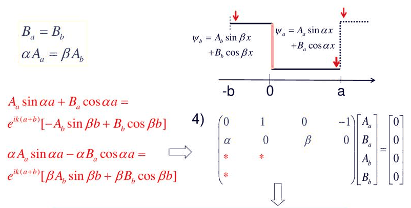
Slide 16: the determinant condition — Slide 16: the 4×4 system and its determinant condition, written with $\xi = E/U_0$ and $\alpha_0 = \sqrt{2mU_0}/\hbar$.

Working out the determinant gives

\det = -2\alpha\beta\,e^{ikL}\left[f(E) - \cos kL\right], \qquad f(E) = \cos\alpha a\,\cos\beta b - \frac{\alpha^2 + \beta^2}{2\alpha\beta}\sin\alpha a\,\sin\beta b .

Below the barrier top, with $\beta = i\gamma$ and $\xi = E/U_0$, this is the slide's form

\cos kL = \cos\!\left(\alpha_0a\sqrt{\xi}\right)\cosh\!\left(\alpha_0b\sqrt{1-\xi}\right) + \frac{1 - 2\xi}{2\sqrt{\xi(1-\xi)}}\sin\!\left(\alpha_0a\sqrt{\xi}\right)\sinh\!\left(\alpha_0b\sqrt{1-\xi}\right),

the Kronig–Penney equation. The factorization is checked numerically below at random energies and wave numbers.

Code45 lines · cell 7

def bc_matrix(E, k):
    """Rows: ψ and ψ' at x = 0; ψ and ψ' at x = a matched to x = -b times e^{ikL}.

    Unknowns A_a, B_a, A_b, B_b."""
    al, be, p = np.sqrt(M * E / H2M0 + 0j), np.sqrt(M * (E - U0) / H2M0 + 0j), np.exp(1j * k * L)
    return np.array(
        [
            [0, 1, 0, -1],
            [al, 0, -be, 0],
            [np.sin(al * A), np.cos(al * A), p * np.sin(be * B), -p * np.cos(be * B)],
            [al * np.cos(al * A), -al * np.sin(al * A), -p * be * np.cos(be * B), -p * be * np.sin(be * B)],
        ]
    )


def kp_f(E):
    """Right-hand side f(E) of cos kL = f(E); real for real E, below and above the barrier top."""
    al, be = np.sqrt(M * E / H2M0 + 0j), np.sqrt(M * (E - U0) / H2M0 + 0j)
    return (
        np.cos(al * A) * np.cos(be * B) - (al**2 + be**2) / (2 * al * be) * np.sin(al * A) * np.sin(be * B)
    ).real


def kp_slide(xi):
    """The slide's form with ξ = E/U0 < 1."""
    a0 = np.sqrt(M * U0 / H2M0)
    sa, sb = a0 * A * np.sqrt(xi), a0 * B * np.sqrt(1 - xi)
    return np.cos(sa) * np.cosh(sb) + (1 - 2 * xi) / (2 * np.sqrt(xi * (1 - xi))) * np.sin(sa) * np.sinh(sb)


rng = np.random.default_rng(1)
worst = 0.0
for E, k in zip(rng.uniform(0.01, 0.8, 200), rng.uniform(-np.pi / L, np.pi / L, 200)):
    al, be = np.sqrt(M * E / H2M0 + 0j), np.sqrt(M * (E - U0) / H2M0 + 0j)
    predicted = -2 * al * be * np.exp(1j * k * L) * (kp_f(E) - np.cos(k * L))
    worst = max(worst, abs(np.linalg.det(bc_matrix(E, k)) - predicted) / abs(predicted))
print(
    "det(4×4) against −2αβ e^(ikL) [f(E) − cos kL], 200 random (E, k): largest relative difference "
    f"{worst:.1e}"
)
xi = np.linspace(0.01, 0.99, 99)
print(
    "slide's ξ form against f(E) below the top: largest difference "
    f"{np.abs(kp_slide(xi) - kp_f(xi * U0)).max():.1e}"
)

det(4×4) against −2αβ e^(ikL) [f(E) − cos kL], 200 random (E, k): largest relative difference 1.7e-14
slide's ξ form against f(E) below the top: largest difference 3.6e-15

The determinant of the lecture's 4×4 matrix equals $-2\alpha\beta e^{ikL}[f(E) - \cos kL]$ to round-off at every tested point, and the slide's $\xi$ form is the same function below the barrier top. The "reasonably horrendous" result, in Klimeck's words, is a single real function $f(E)$ compared with $\cos kL$.

4. Bands from the Kronig–Penney equation and from open-nemo#

Since $|\cos kL| \le 1$, real $k$ exists only where $|f(E)| \le 1$: these energies form the bands. Inverting gives $k(E) = \arccos(f(E))/L$, the band structure. The same bands follow from the discretized Hamiltonian of one cell, used as a periodic lead by nemo.lead_bands. A third, independent check is the transfer matrix of Lecture 6.1: for one period, $\cos kL = \tfrac12\operatorname{Tr}M$.

Code61 lines · cell 9

from scipy.optimize import brentq

lead = nemo.Lead(h, V)
bs = nemo.lead_bands(lead, npts=201, period=L)
kq = bs["k"][:, 0]

E = np.linspace(0.001, 0.8, 8000)
f = kp_f(E)
allowed = np.abs(f) <= 1
edges = E[np.nonzero(np.diff(allowed.astype(int)))[0]]
edges = [brentq(lambda e: abs(kp_f(e)) - 1, e0 - 2e-4, e0 + 2e-4) for e0 in edges]
print("band edges from |f(E)| = 1 (eV):     ", np.round(edges, 4))
print(
    "band edges from open-nemo, k = 0 and π/L:",
    np.round(
        np.sort(np.concatenate([lead.bands(np.array([0.0]))[0][:3], lead.bands(np.array([np.pi]))[0][:3]])), 4
    ),
)


def cell_transfer_trace(E):
    """½ Tr of the one-period transfer matrix (well then barrier), Lecture 6.1 conventions."""
    al, be = np.sqrt(M * E / H2M0 + 0j), np.sqrt(M * (E - U0) / H2M0 + 0j)

    def layer(q, d):  # propagates (ψ, ψ') across a layer of width d
        return np.array([[np.cos(q * d), np.sin(q * d) / q], [-q * np.sin(q * d), np.cos(q * d)]])

    return 0.5 * np.trace(layer(be, B) @ layer(al, A)).real


print(
    f"½ Tr M against f(E) on 50 energies: largest difference "
    f"{max(abs(cell_transfer_trace(e) - kp_f(e)) for e in np.linspace(0.01, 0.8, 50)):.1e}"
)

fig, (a1, a2) = plt.subplots(1, 2, figsize=(11, 4.5), sharey=True)
a1.plot(f, E, **style.series())
a1.axvspan(-1, 1, color=style.CONTEXT, alpha=0.15, lw=0)
a1.set(
    xlabel="f(E) = cos kL", ylabel="energy (eV)", xlim=(-4, 4), ylim=(0, 0.8), title="Kronig–Penney function"
)
kE = np.where(allowed, np.arccos(np.clip(f, -1, 1)) / L, np.nan)
a2.plot(
    kE * L / np.pi, E, **style.series("reference"), label="Kronig–Penney: k = arccos f(E) / L"
)
for n in range(4):
    a2.plot(
        kq * L / np.pi,
        bs["energies"][:, n],
        ".",
        ms=2,
        **style.series(),
        label="open-nemo lead_bands" if n == 0 else None,
    )
for ax in (a1, a2):
    for e in edges:
        ax.axhline(e, color=style.CONTEXT, lw=0.5, ls=":")
a2.axhline(U0, color=style.CONTEXT, lw=0.8)
a2.set(xlabel="k L / π", xlim=(-1, 1), title=f"a = {A} nm, b = {B} nm, U0 = {U0} eV")
a2.legend(frameon=False, fontsize=8, loc="center right")
fig.tight_layout();

band edges from |f(E)| = 1 (eV):      [0.0617 0.0961 0.2399 0.3823 0.5287]
band edges from open-nemo, k = 0 and π/L: [0.0617 0.0961 0.2399 0.3822 0.5286 0.8521]
½ Tr M against f(E) on 50 energies: largest difference 8.9e-16

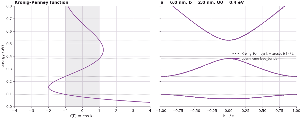
Figure computed by the notebook with open-nemo

Where the curve $f(E)$ lies inside the grey strip $|f| \le 1$ there are Bloch states; where it leaves the strip there are none. The Kronig–Penney equation, the one-period transfer matrix and the discretized Hamiltonian give the same bands, the last within the small grid error of the 0.05 nm spacing. The two bands below the barrier top are those found with transmission through 19 barriers in Lecture 6.4 (0.062–0.096 eV and 0.240–0.382 eV). Above the barrier top the bands continue; the gap above the top (0.382–0.529 eV) is as wide as the first. Lecture 7.2 reads this figure in detail.

5. Exploration: complex wave numbers in the gaps#

In a gap $|f(E)| > 1$, and $\cos kL = f$ has no real solution. It has complex ones: $k = i\kappa$ where $f > 1$, and $k = \pi/L + i\kappa$ where $f < -1$, with

\kappa L = \operatorname{arccosh}|f(E)|.

The wave then decays by $e^{-\kappa L}$ per period; these evanescent Bloch states are what made the transmission through $N$ barriers in the gaps fall exponentially with $N$ (Lecture 6.4). nemo.complex_bands computes them from the same lead.

Code21 lines · cell 11

Eg = np.linspace(0.005, 0.6, 300)
cb = nemo.complex_bands(lead, Eg, period=L)
kappa_nemo = np.nanmin(np.abs(cb["k_imag"]), axis=1)  # slowest-decaying mode
fg = kp_f(Eg)
kappa_kp = np.where(np.abs(fg) > 1, np.arccosh(np.maximum(np.abs(fg), 1)) / L, 0.0)
gap = np.abs(fg) > 1.001
print(
    "largest |κ open-nemo − κ Kronig–Penney| in the gaps: "
    f"{np.abs(kappa_nemo - kappa_kp)[gap].max():.1e} 1/nm "
    f"(κ up to {kappa_kp.max():.3f} 1/nm)"
)
i = np.argmin(np.abs(Eg - 0.17))
print(
    f"at {Eg[i]:.3f} eV (first gap): κ = {kappa_kp[i]:.3f} 1/nm, decay per period e^(-κL) = "
    f"{np.exp(-kappa_kp[i] * L):.3f}"
)
fig, ax = plt.subplots(figsize=(7.5, 4))
ax.plot(kappa_kp, Eg, **style.series("reference"), label="arccosh|f(E)| / L")
ax.plot(kappa_nemo, Eg, **style.series(lw=1), label="open-nemo complex_bands")
ax.set(xlabel="κ = Im k (1/nm)", ylabel="energy (eV)", title="decay constant of the Bloch waves")
ax.legend(frameon=False, fontsize=8);

largest |κ open-nemo − κ Kronig–Penney| in the gaps: 1.0e-03 1/nm (κ up to 0.351 1/nm)
at 0.170 eV (first gap): κ = 0.160 1/nm, decay per period e^(-κL) = 0.278

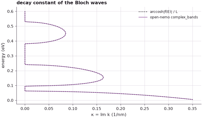
In each gap $\kappa$ rises from zero at one band edge to a maximum and falls back to zero at the next edge, and open-nemo's complex band structure follows the analytic $\operatorname{arccosh}$ to 0.001 nm$^{-1}$. In the middle of the first gap the amplitude of the wave drops to a fraction $e^{-\kappa L}$ per period, which is why a few periods of a superlattice already block electrons in a gap. The bands and the gaps are two faces of the same equation: real $k$ where $|f| \le 1$, complex $k$ where $|f| > 1$.

Summary#

A long periodic structure is modelled as infinitely repeated, with the smallest unit cell of period $L = a + b$.
Bloch's theorem: $\psi(x + L) = e^{ikL}\psi(x)$. A ring of $N$ cells quantizes $k = 2\pi n/(NL)$ in $[-\pi/L, \pi/L)$, $N$ states per band; numerically the ring problem splits into $N$ one-cell problems with identical eigenvalues.
The boundary conditions of one cell, the last two carrying the phase $e^{ikL}$, form a 4×4 system; its determinant is $-2\alpha\beta e^{ikL}[f(E) - \cos kL]$.
Bands are where $|f(E)| \le 1$ (Kronig–Penney equation, also $\tfrac12\operatorname{Tr}M$ of one period); in the gaps $k$ is complex with $\kappa L = \operatorname{arccosh}|f|$.

Exercises#

Repeat the ring test of Section 2 with $N = 5$ (odd). Which values of $n$ are allowed, and is the zone-boundary state $k = -\pi/L$ still present?
Take the limit $U_0 \to 0$ in $f(E)$ and show that the bands become the free-electron parabola folded into $[-\pi/L, \pi/L]$.
Take the limit $b \to 0$, $U_0 \to \infty$ with $U_0b$ fixed (a Dirac comb) and derive the simplified Kronig–Penney equation $\cos kL = \cos\alpha a + P\,\sin\alpha a/(\alpha a)$. Identify $P$.
Give the barrier its own mass ($0.092\,m_0$). Which entries of bc_matrix change (hint: $\psi'/m$ is continuous), and how does $f(E)$ change? Compare with lead_bands of a cell with two materials.