

Lecture 11.3
Resonant tunneling diodes with relaxation in the reservoirs
In the lecture
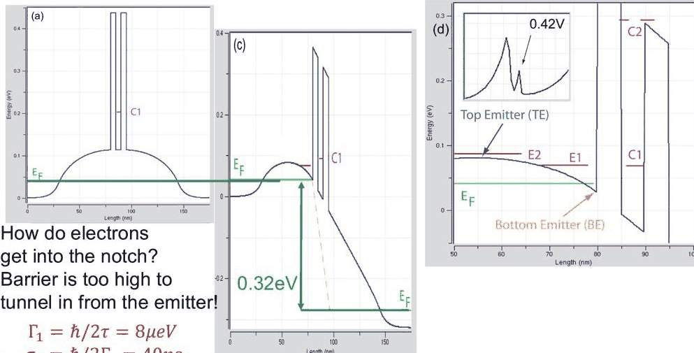
- the practical problem with the sharp emitter states of lecture 11.2: electrons cannot tunnel into the notch, and lifetimes of tens of picoseconds are unphysical in a heavily doped emitter
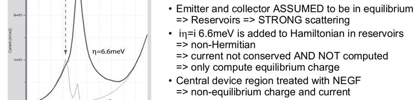
- NEMO's relaxation in the reservoirs: an imaginary potential \(-i\eta\) with \(\eta = 6.6\) meV in the equilibrium emitter and collector, and the partitioning of the device into reservoirs and a central non-equilibrium (NEGF) region
- what relaxation does: emitter states broadened beyond 6.6 meV, the central resonance almost unchanged, a single I–V peak with more current and more valley current, Urbach tails below the band edge
- an industrial example from 1994–95: a GaAs/Al${0.4}$Ga${0.6}$As RTD where different contact treatments disagree by orders of magnitude, and an InP optical switch that NEMO matched
- the reduction of the scattering domain that the partitioning makes possible
In this notebook
uses the realistic-doping RTD of lecture 11.2 and computes the Thomas–Fermi I–V with and without reservoir relaxation (nemo.thomas_fermi_iv(relaxation=...)), the resonance widths with the reservoir broadening (nemo.resonances(reservoir=...)), the transmission and current spectrum at 0.32, 0.42 and 0.76 V with reservoir_transmission, the share of current carried by the central resonance and by energies below the emitter band edge, the dependence on \(\eta\), and the cost argument for a small scattering domain.
Run it on your own machine
The notebook needs open-nemo (Python ≥ 3.10 and a C++20 compiler; BLAS/LAPACK).
git clone https://github.com/denphi/open-nemo.git && cd open-nemo
python3 -m venv .venv && source .venv/bin/activate
pip install -e ".[notebooks]"
jupyter lab From_Atoms_to_Devices/06_resonant_tunneling_diodes/11_3_relaxation_in_the_reservoirs.ipynbCode
import numpy as np
import matplotlib.pyplot as plt
import opennemo as nemo
from opennemo.visualization import style

style.use(notebook=True)
H2M0 = nemo.core.units.HBAR2_2M0          # ħ²/2m₀ = 0.0381 eV nm²
EM = nemo.structures.materials.EffectiveMassMaterial
1. A practical problem with the emitter states#
Lecture 11.2 found quasi-bound states E1 and E2 in the triangular notch in front of the first barrier. The width of E1 fell exponentially with bias, to about 8 µeV in the lecture's example, a lifetime of 40 ps. The lecturer now asks two questions. First, how do electrons get into the notch at all? The hump between the notch and the emitter contact is low but tens of nanometres long, too thick to tunnel through in any reasonable time. Second, can an electron really stay coherently in the notch for 40 ps? The notch holds a sheet density of \(10^{10}\) to \(10^{12}\) electrons per cm$^2$. Electrons at that density scatter off each other and off phonons on time scales of about \(\tau = 50\) fs, so the states must be broadened by about
nearly a thousand times more than the coherent calculation gives. The 8 µeV line is, in the lecturer's words on the slide, "incorrect physics".
The first cell rebuilds the device of lecture 11.2 (30 nm \(10^{18}\) cm$^{-3}$ contacts, 50 nm spacers, 4/5/4 nm Al${0.3}$Ga${0.7}$As/GaAs/Al${0.3}$Ga${0.7}$As) and checks the sheet density in the notch.
Code
from opennemo.solvers.reservoir import reservoir_transmission

x_al = 0.3
gaas = EM("GaAs", 0.067, 12.9, conduction_band_edge=0.0)
algaas = EM("Al0.3Ga0.7As", 0.067 + 0.083 * x_al, 12.9 - 2.84 * x_al, conduction_band_edge=0.324)
layers = [
    nemo.Layer(gaas, 30, donors=1e18, name="emitter contact"),
    nemo.Layer(gaas, 50, donors=1e15, name="emitter spacer"),
    nemo.Layer(algaas, 4, name="barrier"),
    nemo.Layer(gaas, 5, name="well"),
    nemo.Layer(algaas, 4, name="barrier"),
    nemo.Layer(gaas, 50, donors=1e15, name="collector spacer"),
    nemo.Layer(gaas, 30, donors=1e18, name="collector contact"),
]
rtd = nemo.Heterostructure1D(layers, spacing=0.25, terminal_layers=(2, 2))
x, XB1 = rtd.x, 80.0
emitter = x < XB1
T, ETA = 300, 0.0066
V = np.round(np.arange(0.0, 0.8001, 0.01), 3)
ballistic = nemo.thomas_fermi_iv(rtd, V, T, charge="all", relaxation=None)
relaxed = nemo.thomas_fermi_iv(rtd, V, T, charge="all", relaxation=ETA, relaxation_decay=ETA)
EF = float(np.atleast_1d(relaxed["mu_left"])[0])
Ec = rtd.band_edge[None, :] + relaxed["potential"]
print(
    "largest potential difference between the two runs:",
    f"{np.abs(ballistic['potential'] - relaxed['potential']).max():.1e} eV",
)

for v in (0.32, 0.42, 0.76):
    i = int(np.argmin(abs(V - v)))
    ec = Ec[i]
    itop = int(np.argmax(np.where(emitter, ec, -1)))
    notch = emitter & (np.arange(len(x)) > itop)
    sheet = relaxed["electron_density"][i][notch].sum() * rtd.spacing * 1e-7  # cm^-2
    print(f"{v:.2f} V: sheet density between the emitter top and the barrier {sheet:.2g} cm^-2")
print(f"hbar/(2 x 50 fs) = {6.582e-16 / (2 * 50e-15) * 1e3:.2f} meV")
largest potential difference between the two runs: 0.0e+00 eV
0.32 V: sheet density between the emitter top and the barrier 3.4e+11 cm^-2
0.42 V: sheet density between the emitter top and the barrier 4.4e+11 cm^-2
0.76 V: sheet density between the emitter top and the barrier 7.6e+11 cm^-2
hbar/(2 x 50 fs) = 6.58 meV
The Thomas–Fermi potential does not depend on the relaxation (the charge model is the same), so both runs share one potential and differ only in how the current is computed. The notch holds a few times \(10^{11}\) electrons per cm$^2$, inside the range the lecture quotes.
2. Relaxation in the reservoirs#
NEMO (Klimeck et al., APL 1994/95) introduced a simple fix. The emitter and the collector are assumed to be in equilibrium: they are reservoirs in which so much scattering happens that the electrons are thermalised to the Fermi level of their contact. That scattering is not computed; its effect on the states is imitated by adding an imaginary potential, an optical potential, to the Hamiltonian of the reservoir sites,
A state that lives in the reservoir then decays in time and its line has a width of at least of order \(\eta\). Consequences of this construction, as the lecture lists them:
- The reservoir Hamiltonian is non-Hermitian, so current is not conserved there. The reservoirs are only used to compute the (equilibrium) charge, never the current.
- The current is computed in a central region, treated with the non-equilibrium Green function (NEGF) method, which sees the broadened, thermalised states of the reservoirs through their self-energies.
- \(\eta\) is constant above the local band edge and decays below it (here exponentially over 6.6 meV), which gives the density of states an Urbach-like tail into the gap.
In open-nemo the reservoirs are the terminal_layers of the heterostructure (here contact plus spacer on
each side), and thomas_fermi_iv(relaxation=η, relaxation_decay=...) or
reservoir_transmission(device, potential, eta, decay) apply the model. The central region is the double
barrier, extended by NEMO's default non_equilibrium=(-1, 0) by one monolayer into the emitter.
3. Resonance widths with relaxation#
nemo.resonances(..., reservoir=(η, decay, model, non_equilibrium)) adds the same relaxation to the
open-system eigenproblem, so the widths below include the reservoir broadening. The cell traces the
central resonance C1 and the lowest notch state E1 with and without it.
Code
RES = (ETA, ETA, "exponential", (-1, 0))


def c1_e1(i, reservoir):
    """(E, width) of the central state C1 and of the lowest notch state E1 at bias index i."""
    ec = Ec[i]
    r = nemo.resonances(
        rtd,
        potential=relaxed["potential"][i],
        confinement_region=(-160, 0),
        emin=ec[emitter][-1] - 0.005,
        emax=0.3,
        reservoir=reservoir,
    )
    e, g, x0 = r["energy"], r["width"], r["x0"]
    well = np.flatnonzero((x0 > XB1 + 3) & (x0 < XB1 + 10) & (g < 3e-3))
    c = well[np.argmin(e[well])] if len(well) else None
    lim = 3e-3 if reservoir is None else 0.05  # ballistic E1 is sharp; with relaxation it is >= eta
    notch = np.flatnonzero((x0 < XB1 + 3) & (e < ec[emitter].max()) & (g < lim))
    n = notch[np.argmin(e[notch])] if len(notch) else None
    pick = lambda k: (e[k], g[k]) if k is not None else (np.nan, np.nan)
    return pick(c) + pick(n)


IT = range(4, len(V), 2)
tab = {name: np.array([c1_e1(i, res) for i in IT]) for name, res in (("ballistic", None), ("relaxed", RES))}
VT = V[list(IT)]
for v in (0.32, 0.5, 0.6):
    k = int(np.argmin(abs(VT - v)))
    b, r = tab["ballistic"][k], tab["relaxed"][k]
    print(
        f"{VT[k]:.2f} V: width C1 {1e3 * b[1]:.2f} -> {1e3 * r[1]:.2f} meV;  "
        f"width E1 {1e3 * b[3]:.3g} -> {1e3 * r[3]:.3g} meV"
    )
0.32 V: width C1 0.46 -> 0.43 meV;  width E1 0.0711 -> 12 meV
0.50 V: width C1 0.37 -> 0.41 meV;  width E1 0.00433 -> 11.8 meV
0.60 V: width C1 0.41 -> 0.42 meV;  width E1 0.00143 -> 11.7 meV
Code
fig, (a1, a2) = plt.subplots(1, 2, figsize=(10.5, 3.8))
for name, ls in (("ballistic", "--"), ("relaxed", "-")):
    t = tab[name]
    a1.plot(VT, t[:, 0], ls, color="C3", label=f"C1, {name}")
    a1.plot(VT, t[:, 2], ls, color=style.OPEN_NEMO, label=f"E1, {name}")
    a2.semilogy(VT, 1e3 * t[:, 1], ls, color="C3", label=f"C1, {name}")
    a2.semilogy(VT, 1e3 * t[:, 3], ls, color=style.OPEN_NEMO, label=f"E1, {name}")
a2.axhline(1e3 * ETA, color=style.CONTEXT, lw=1, ls=":", label="$\\eta$ = 6.6 meV")
a1.set(xlabel="Bias (V)", ylabel="Energy (eV)", title="C1 and E1 energies")
a2.set(xlabel="Bias (V)", ylabel="Width (meV)", title="C1 and E1 widths")
a1.legend(fontsize=7)
a2.legend(fontsize=7, ncol=2)
fig.tight_layout();
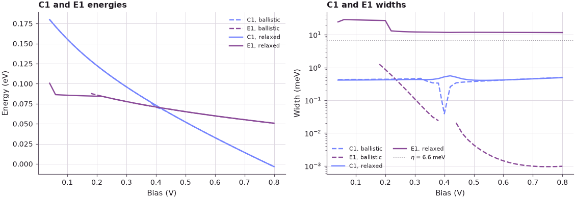
With relaxation the emitter state E1 is never narrower than a little under \(2\eta\): in the reservoir the state decays at the rate \(2\eta/\hbar\), which is the width NEMO reports. The microelectronvolt lines of the coherent calculation are gone. The central resonance C1 lives in the coherent region and keeps its width of about 0.4 meV; only near the crossing with E1, where the two states mix, does it change a little (a small blip, as on the lecture's slide). Now every emitter state is broader than C1: the narrow central resonance is the filter that probes the emitter, and its width limits the current.
4. The I–V characteristic with relaxation#
Code
Jb, Jr = ballistic["current_density"], relaxed["current_density"]
kb, kr = int(np.argmax(Jb)), int(np.argmax(Jr))
print(f"ballistic: peak {Jb[kb]:.0f} A/cm^2 at {V[kb]:.2f} V, current at 0.7 V {Jb[V == 0.7][0]:.0f} A/cm^2")
print(
    f"relaxed:   peak {Jr[kr]:.0f} A/cm^2 at {V[kr]:.2f} V, valley {Jr[kr:].min():.0f} A/cm^2 at "
    f"{V[kr + np.argmin(Jr[kr:])]:.2f} V, current at 0.7 V {Jr[V == 0.7][0]:.0f} A/cm^2"
)

fig, (a1, a2) = plt.subplots(1, 2, figsize=(10, 3.8))
for J, c, lab in ((Jb, style.CONTEXT, "ballistic, $\\eta=0$"), (Jr, style.OPEN_NEMO, "$\\eta$ = 6.6 meV")):
    a1.plot(V, J, color=c, lw=2, label=lab)
    a2.semilogy(V[1:], J[1:], color=c, lw=2, label=lab)
a1.set(xlabel="Bias (V)", ylabel="Current density (A/cm²)", title="Thomas–Fermi potential, 300 K")
a2.set(xlabel="Bias (V)", ylabel="Current density (A/cm²)", title="log scale")
a1.legend();
ballistic: peak 2403 A/cm^2 at 0.32 V, current at 0.7 V 300 A/cm^2
relaxed:   peak 6935 A/cm^2 at 0.43 V, valley 1263 A/cm^2 at 0.80 V, current at 0.7 V 1557 A/cm^2
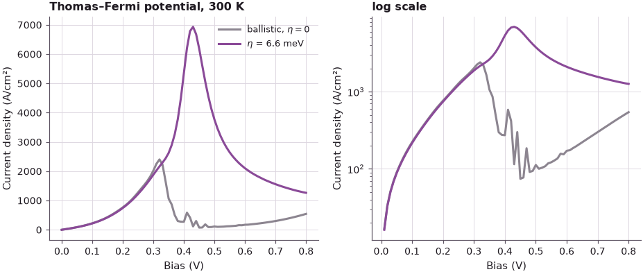
Relaxation changes the I–V qualitatively. The two sharp peaks of the coherent calculation merge into one broad peak at a higher bias, with a peak current almost three times larger, and the valley current is several times higher. The narrow emitter states that limited the current in the coherent picture are now broadened and filled from the thermalised reservoir, so C1 sees a continuous, much better supply.
5. Transmission and current spectrum at three biases#
The lecture compares \(T(E)\) and the current density with and without \(\eta\) at 0.32 V (C1 aligned with
E2), 0.42 V (C1 aligned with E1) and 0.76 V (deep in the valley). With relaxation, reservoir_transmission
returns the generalised transmission of the partitioned device; the current is again the Tsu–Esaki
integral of it. The energy grid starts 0.15 eV below the emitter contact band edge to catch the current
that the Urbach tails let through.
Code
tr = nemo.Transport(rtd.hamiltonian)
kT = 8.617e-5 * T


def spectra(v):
    i = int(np.argmin(abs(V - v)))
    u = relaxed["potential"][i]
    r0 = nemo.resonances(rtd, potential=u, emin=-v, emax=0.3)
    c1, g1 = r0["energy"][0], r0["width"][0]
    rn = nemo.resonances(
        rtd, potential=u, confinement_region=(-160, 0), emin=Ec[i][emitter][-1] - 0.005, emax=0.3
    )
    seeds = [e + max(w, 1e-7) * np.linspace(-15, 15, 151) for e, w in zip(rn["energy"], rn["width"])]
    E = np.unique(np.concatenate([np.linspace(-0.15, EF + 15 * kT, 4000)] + seeds))
    E = E[E < EF + 15 * kT]
    out = dict(E=E, c1=c1, i=i)
    for name, t in (
        ("ballistic", tr.transmission(E, potential=u)),
        ("relaxed", reservoir_transmission(rtd, u, eta=ETA, decay=ETA)(E)),
    ):
        Je = rtd.current_spectrum(E, t, EF, EF - v, T)
        J = rtd.current_density(E, t, EF, EF - v, T)
        cum = np.concatenate([[0], np.cumsum(0.5 * (Je[1:] + Je[:-1]) * np.diff(E))]) / J
        at = lambda e0: cum[np.argmin(abs(E - e0))]
        out[name] = dict(T=t, J=J, cum=cum, nearC1=at(c1 + 3e-3) - at(c1 - 3e-3), below=at(0.0))
    return out


SP = {v: spectra(v) for v in (0.32, 0.42, 0.76)}
for v, s in SP.items():
    for name in ("ballistic", "relaxed"):
        d = s[name]
        print(
            f"{v:.2f} V {name:9s}: J = {d['J']:7.0f} A/cm^2, within ±3 meV of C1 {100 * d['nearC1']:5.1f}%, "
            f"below the emitter contact band edge {100 * d['below']:.2f}%"
        )
0.32 V ballistic: J =    2425 A/cm^2, within ±3 meV of C1  95.5%, below the emitter contact band edge 0.00%
0.32 V relaxed  : J =    2163 A/cm^2, within ±3 meV of C1  94.8%, below the emitter contact band edge 0.00%
0.42 V ballistic: J =     510 A/cm^2, within ±3 meV of C1  86.8%, below the emitter contact band edge 0.00%
0.42 V relaxed  : J =    6785 A/cm^2, within ±3 meV of C1  96.0%, below the emitter contact band edge 0.00%
0.76 V ballistic: J =     433 A/cm^2, within ±3 meV of C1   0.0%, below the emitter contact band edge 0.00%
0.76 V relaxed  : J =    1358 A/cm^2, within ±3 meV of C1  59.4%, below the emitter contact band edge 0.46%
Code
fig, axes = plt.subplots(2, 3, figsize=(11, 6.4), sharey=True)
for col, (v, s) in zip(axes.T, SP.items()):
    for name, c, ls in (("ballistic", style.CONTEXT, "--"), ("relaxed", style.OPEN_NEMO, "-")):
        col[0].semilogx(s[name]["T"], s["E"], ls, color=c, label=name)
        col[1].plot(s[name]["cum"], s["E"], ls, color=c, label=name)
    for a in col:
        a.axhline(s["c1"], color="C3", lw=0.8, ls=":")
        a.axhline(0, color=style.REFERENCE, lw=0.6)
    col[0].set(title=f"{v:.2f} V", xlim=(1e-9, 2), xlabel="$T(E)$")
    col[1].set(xlabel="running integral $I(E)/I$")
axes[0, 0].set(ylabel="Energy (eV)", ylim=(-0.08, 0.35))
axes[1, 0].set(ylabel="Energy (eV)")
axes[0, 0].legend(fontsize=8)
fig.suptitle("Transmission and running current integral (dotted: C1; solid black: emitter contact band edge)")
fig.tight_layout();
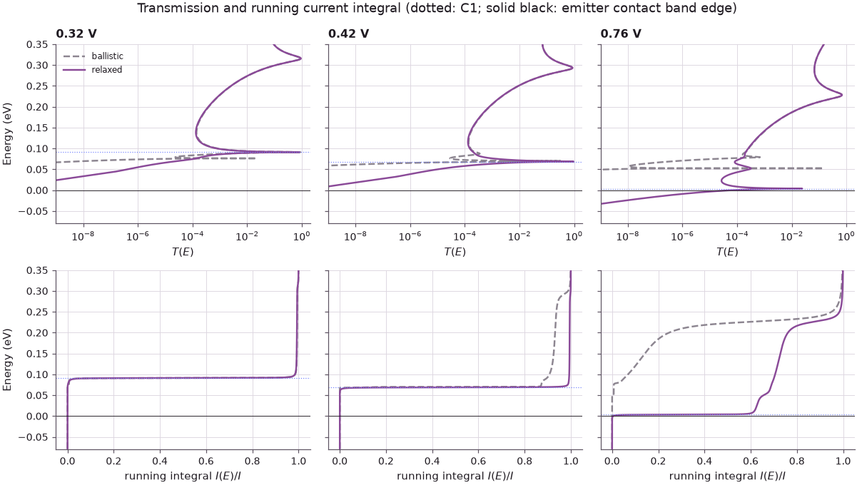
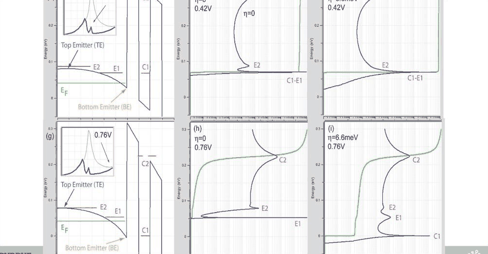
At 0.32 and 0.42 V the sharp, separate transmission features of the coherent calculation are smoothed into one broad line, and the current still flows almost entirely through C1. In the valley (0.76 V) the difference is large: without relaxation C1 lies below every emitter state and only the far-off background carries current; with relaxation a large part of the current still flows through C1, because the broadened emitter states, with their tails, reach down to it. The share of current from energies below the emitter contact band edge is small but no longer zero: those are the Urbach tails built into the decaying \(\eta\). The lecture's device has about 20% of its valley current through C1; in this device the share is larger because C1 is closer to the emitter states at 0.76 V.
6. How strong is the relaxation? Do not tune it#
The lecturer is explicit that \(\eta\) is an empirical parameter that he does not adjust to fit measurements: for typical InGaAs/InAlAs and GaAs/AlGaAs RTDs NEMO uses 6.6 meV (\(\tau=0.05\) ps) and keeps it. As an exercise he suggests changing it to see what happens:
Code
fig, ax = plt.subplots(figsize=(6, 3.8))
for eta, c in zip((0.002, 0.0066, 0.02), style.sweep(3)):
    J = nemo.thomas_fermi_iv(rtd, V, T, charge="all", relaxation=eta, relaxation_decay=eta)["current_density"]
    k = int(np.argmax(J))
    print(
        f"eta = {1e3 * eta:4.1f} meV: peak {J[k]:6.0f} A/cm^2 at {V[k]:.2f} V, "
        f"valley {J[k:].min():5.0f} A/cm^2, PVR {J[k] / J[k:].min():.1f}"
    )
    ax.plot(V, J, color=c, lw=2, label=f"$\\eta$ = {1e3 * eta:.1f} meV")
ax.plot(V, Jb, "--", color=style.CONTEXT, label="ballistic")
ax.set(xlabel="Bias (V)", ylabel="Current density (A/cm²)", title="Sensitivity to the reservoir relaxation")
ax.legend();
eta =  2.0 meV: peak  10514 A/cm^2 at 0.42 V, valley   676 A/cm^2, PVR 15.6
eta =  6.6 meV: peak   6935 A/cm^2 at 0.43 V, valley  1263 A/cm^2, PVR 5.5
eta = 20.0 meV: peak   5531 A/cm^2 at 0.54 V, valley  3650 A/cm^2, PVR 1.5
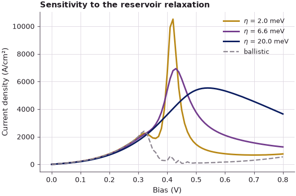
The choice matters. A smaller \(\eta\) (2 meV) gives a higher peak and a lower valley, a peak-to-valley ratio of 15.6; the standard 6.6 meV gives 5.5; a larger \(\eta\) (20 meV) moves the peak to higher bias and fills the valley, a ratio of only 1.5. Precisely because the valley current is so sensitive to \(\eta\), fitting it to a measurement would hide whatever physics is actually missing (contacts, band structure); a fixed, physically motivated value keeps the model honest.
7. Why the contacts matter: an industrial RTD in 1994#
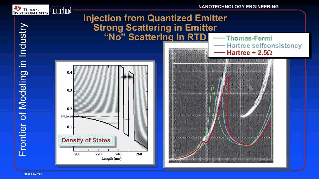
The lecturer next shows work from his time at Texas Instruments and UT Dallas: a "benign" GaAs/Al${0.4}$Ga${0.6}$As RTD with 5 nm barriers and a 5 nm well, 18 nm undoped spacers, 200 nm buffers doped to \(2\times10^{15}\) cm$^{-3}$ and 20 nm contacts doped to \(2\times10^{18}\) cm$^{-3}$. The goal was a peak-to-valley ratio above 1000 (typical was 3), and the whole field was convinced that the valley current came from scattering inside the RTD: electrons emit a phonon in the well and leave below the resonance. That turned out to be wrong, because the treatment of the contacts and the band structure were missing.
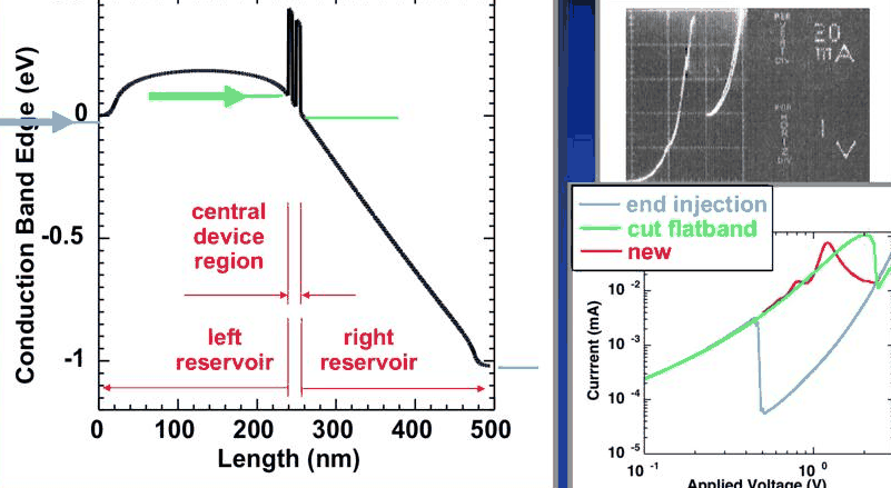
Is this a 15 nm device or a 500 nm device? Three ways to model it give very different answers on the same log–log I–V plot:
- Flat-band end injection (the 1994 state of the art): flat contacts attached to the two ends of the structure and electrons shot coherently through the whole potential.
- Cut flat band: compute the potential of the whole structure, then attach a flat-band contact right before the notch and inject from there.
- Partitioned reservoirs (NEMO): the device split into an emitter reservoir, a central region and a collector reservoir with relaxation, as above.
The first two differ by an order of magnitude in the peak voltage and two orders of magnitude in the peak current, although both give a nice N-shaped curve. The third overlaps the measured curve, including a small shoulder that comes from C1 probing a state of the emitter notch.
The Thomas–Fermi model is not the end of the story. A Hartree (quantum self-consistent) potential bends the I–V over towards higher bias, a series resistance in the contacts bends it further, and the valley current needs a band structure beyond the single-band effective mass approximation, which later lectures cover.
8. Complicated emitters, and a smaller scattering domain#
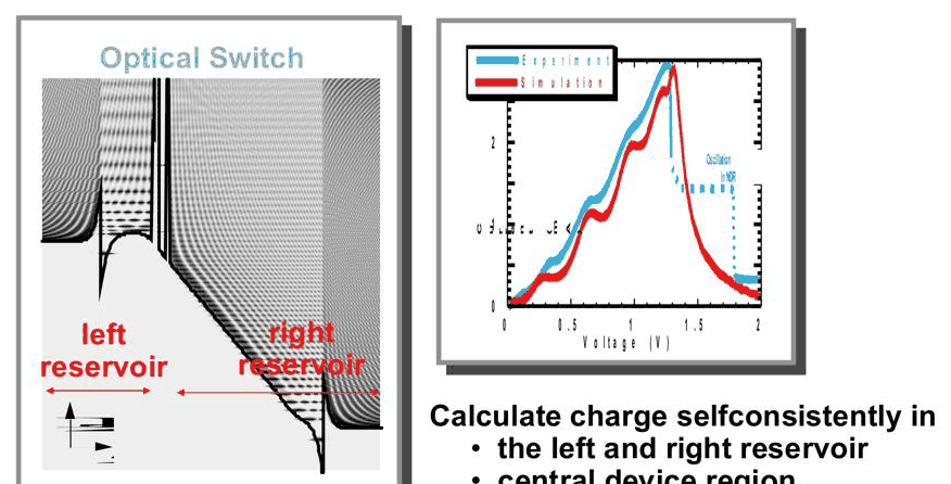
The partitioning handles emitters that wave-function methods cannot. The lecturer's example is an InP RTD with an optical window used as an optical switch (Klimeck et al., Device Research Conference 1995): the emitter contains a triangular well and many more quantised states, and the NEMO simulation, with the charge computed self-consistently in both reservoirs and the central region, reproduces the measured shoulders.
The partitioning has a second benefit. Scattering inside the device (phonons, alloy disorder, interface roughness) couples sites to each other, and the cost of NEGF with scattering grows from \(N^2\) to \(N^3\) in the number of sites \(N\) of the non-equilibrium region, against linear cost for the coherent recursive Green function algorithm of lecture 12. With the reservoirs assumed in equilibrium, only the central region needs the expensive treatment:
Code
from opennemo.models.ema import _active_region

first, last = _active_region(rtd, (-1, 0))
n_all, n_mid = rtd.num_sites, last - first + 1
print(
    f"whole device {n_all} sites, central non-equilibrium region {n_mid} sites "
    f"({x[first]:.2f} to {x[last]:.2f} nm)"
)
print(f"N^3 cost ratio of scattering over the whole device vs the central region: {(n_all / n_mid) ** 3:.0f}")
whole device 692 sites, central non-equilibrium region 53 sites (79.88 to 92.88 nm)
N^3 cost ratio of scattering over the whole device vs the central region: 2226
Summary#
- Triangular notches in the emitter confine electrons. Without relaxation their states have lifetimes of tens of picoseconds and widths of microelectronvolts, which makes no physical sense in an emitter with \(10^{11}\) electrons per cm$^2$ that scatter on a 50 fs time scale.
- NEMO adds an empirical relaxation \(-i\eta\) (\(\eta = \hbar/2\tau = 6.6\) meV) in the emitter and collector, which are assumed to be equilibrium reservoirs. The reservoirs are non-Hermitian and used only for the charge; the current is computed in the central NEGF region, which sees thermalised, broadened states.
- With relaxation the emitter states are broader than about 2η, the central resonance keeps its 0.4 meV, the I–V has a single larger peak and more valley current, and some current flows below the emitter band edge through Urbach tails.
- Contact treatment changes simulated RTD currents by orders of magnitude; together with band structure it, not scattering in the well, explained the valley currents of real devices.
- \(\eta\) is not a fitting parameter. The partitioning also shrinks the region where costly scattering calculations are needed.
Exercises#
- Change
relaxation_decaytoNone(constant \(\eta\), no decay below the band edge) and recompute the relaxed I–V and the share of current below the emitter band edge at 0.76 V. - Run
thomas_fermi_ivwithnon_equilibrium=(-20, 0), moving five nanometres of the emitter notch into the coherent region. How do the I–V and the E1 width change? - Add a series resistance: with a specific contact resistance \(r_s\) (Ω cm²), the external voltage is \(V_{\text{ext}} = V + J r_s\). Plot \(J\) against \(V_{\text{ext}}\) for \(r_s = 10^{-5}\) Ω cm² and explain why the peak moves and the NDR region can become multivalued.
- Repeat the comparison at 77 K. Which features of the ballistic I–V survive the relaxation?
Further reading#
- Lecture 11.2: RTDs with realistic doping profiles
- Lecture 11.4: Hartree self-consistency
- RTD tutorial
- RTD scattering models: relaxation, Büttiker probes, phonons
- NEMO-1D benchmark: self-consistent RTD
- G. Klimeck, R. Lake, R. C. Bowen, W. R. Frensley and T. S. Moise, "Quantum device simulation with a generalized tunneling formula", Appl. Phys. Lett. 67, 2539 (1995).
- R. Lake, G. Klimeck, R. C. Bowen and D. Jovanovic, "Single and multiband modeling of quantum electron transport through layered semiconductor devices", J. Appl. Phys. 81, 7845 (1997).