Course/03 · Tunneling and band structure

ECE 606 Lecture 7.3

Band properties: wave packets, effective mass, electrons and holes

In the lecture

a wave packet built from two (or many) Bloch waves moves with the group velocity $v = (1/\hbar)\,dE/dk$
a force changes the crystal momentum, $\hbar\,dk/dt = F$, which defines the effective mass $1/m^* = (1/\hbar^2)\,d^2E/dk^2$
the effective mass depends on the band and on $k$, and is negative near the top of a band
the effective mass is not essential: for a linear dispersion (graphene) it is undefined, while velocity and the integral description still work
empty and full bands carry no current; partially filled bands do, and a nearly full band is described by its empty states, the holes

In this notebook

computes the group velocity of the Kronig–Penney superlattice of Lectures 7.1 and 7.2 from open-nemo's band structure and checks it against wave packets propagated in time with open-nemo's Hamiltonian, maps $v(k)$ and $m^*(k)$ for three bands, follows packets accelerated by a uniform force through a full Bloch oscillation (including the negative mass at the band top), shows how the effective mass vanishes as a two-band chain becomes gapless, and counts the current of full, partially filled and nearly full bands on a ring of cells.

Run the notebookEvery number and figure on this page comes from it. Change it, rerun it, take it further.

Download .ipynb View on GitHub

Run it on your own machine

The notebook needs open-nemo (Python ≥ 3.10 and a C++20 compiler; BLAS/LAPACK).

git clone https://github.com/denphi/open-nemo.git && cd open-nemo
python3 -m venv .venv && source .venv/bin/activate
pip install -e ".[notebooks]"
jupyter lab From_Atoms_to_Devices/03_tunneling_and_bandstructure/07_3_band_properties.ipynb

Code8 lines · cell 1

import numpy as np
import matplotlib.pyplot as plt
import opennemo as nemo
from opennemo.visualization import style

style.use(notebook=True)
H2M0 = nemo.core.units.HBAR2_2M0          # ħ²/2m₀ = 0.0381 eV nm²
EM = nemo.structures.materials.EffectiveMassMaterial

1. Wave packets and the group velocity#

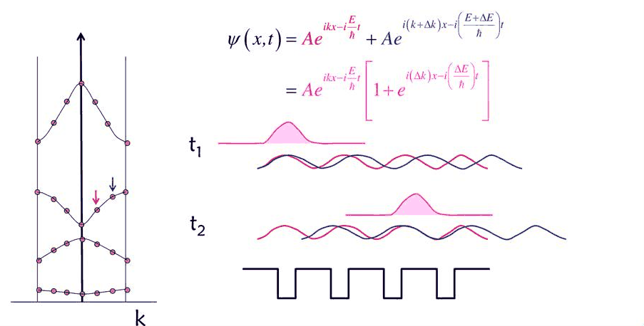
A single Bloch wave $\psi_k(x)e^{-iE(k)t/\hbar}$ is spread over the whole crystal and does not move. A localized electron is a wave packet, a superposition of Bloch waves with nearby $k$. The lecture starts with the simplest case, two waves with wave numbers $k$ and $k + \Delta k$ and energies $E$ and $E + \Delta E$:

\psi(x,t) = Ae^{i(kx - Et/\hbar)}\left[1 + e^{i(\Delta k\,x - \Delta E\,t/\hbar)}\right].

The first factor is the fast carrier; the bracket is a slow envelope (the "signal"). A point of constant envelope phase satisfies $\Delta k\,x - \Delta E\,t/\hbar = \text{const}$, so it moves with

v = \frac{dx}{dt} = \frac{1}{\hbar}\frac{\Delta E}{\Delta k} \;\to\; \frac{1}{\hbar}\frac{dE}{dk},

the group velocity of the band at $k$. It is set by the slope of $E(k)$, not by $E$ itself, and it is zero at the bottom and the top of every band, where the slope vanishes.

Slide 3: wave packet and group velocity — Slide 3: two waves (red and blue) of slightly different $k$ and $E$ add up to a packet whose maximum moves from $t_1$ to $t_2$.

The structure is the GaAs superlattice of Lectures 7.1 and 7.2: wells $a = 6$ nm, barriers $b = 2$ nm and $U_0 = 0.4$ eV, period $L = 8$ nm, mass $m = 0.067\,m_0$. open-nemo provides the Hamiltonian of one cell (h0) and the coupling to the next cell (h1), wrapped in a nemo.Lead; its bands are $E_n(k)$. The group velocity follows either from a numerical derivative of $E_n(k)$ or exactly from the Hellmann–Feynman theorem, $v = \langle u_k|\partial H(k)/\partial k|u_k\rangle/\hbar$, with $H(k) = h_0 + h_1e^{ikL} + h_1^\dagger e^{-ikL}$ and $u_k$ the cell eigenvector.

To test the statement $v = (1/\hbar)\,dE/dk$ the packet is also propagated in time. A chain of 80 cells (640 nm, closed at both ends) is built with nemo.Heterostructure1D, its Hamiltonian is diagonalized once, $H = \sum_n E_n|n\rangle\langle n|$, and any initial state evolves as $\psi(t) = \sum_n c_n e^{-iE_nt/\hbar}|n\rangle$. The initial state is a Bloch function of the first band at $k_0$ times a Gaussian envelope of width $\sigma = 40$ nm. A grid of 0.25 nm keeps the chain at 2560 sites; the bands used for comparison come from the cell on the same grid.

Code79 lines · cell 3

M, A, B, U0 = 0.067, 6.0, 2.0, 0.4
L = A + B
HBAR = nemo.core.units.HBAR * 1e15  # ħ in eV fs, so velocities come out in nm/fs


def superlattice(n_cells, dx, U=U0, m=M):
    """n_cells periods of (well A, barrier B), closed at both ends."""
    w, b = EM("well", m, 12.9), EM("barrier", m, 12.9, conduction_band_edge=U)
    layers = [nemo.Layer(mat, d) for _ in range(n_cells) for mat, d in ((w, A), (b, B))]
    return nemo.Heterostructure1D(layers, spacing=dx)


def cell_lead(dx, U=U0, m=M):
    """One period as a nemo.Lead: h0 from open-nemo's Hamiltonian, h1 the bond to the next cell."""
    h = superlattice(1, dx, U, m).hamiltonian.sparse.dense().real
    V = np.zeros_like(h)
    V[-1, 0] = -H2M0 / (m * dx**2)
    return nemo.Lead(h, V)


def bloch(lead, kL, band=0):
    """Energy, cell eigenvector and Hellmann–Feynman group velocity (nm/fs) at k L = kL."""
    h0, h1 = lead.h0, lead.h1
    e, u = np.linalg.eigh(h0 + h1 * np.exp(1j * kL) + h1.conj().T * np.exp(-1j * kL))
    dH = 1j * L * (h1 * np.exp(1j * kL) - h1.conj().T * np.exp(-1j * kL))
    phi = u[:, band]
    return e[band], phi, (phi.conj() @ dH @ phi).real / HBAR


DXP, NC = 0.25, 80
lead_p = cell_lead(DXP)
chain = superlattice(NC, DXP)
H = chain.hamiltonian.sparse.dense().real
x = chain.x
E_n, P = np.linalg.eigh(H)
print(f"chain: {NC} cells, {H.shape[0]} sites, length {x[-1] + DXP / 2:.0f} nm")
print(f"cell bands at k = 0 (0.25 nm grid): {np.round(lead_p.bands(np.array([0.0]))[0][:3], 4)} eV")


def packet(k0, x0, sigma, band=0, lead=lead_p):
    """Bloch function of `band` at wave number k0 (1/nm) times a Gaussian envelope (σ in nm)."""
    _, phi, _ = bloch(lead, k0 * L, band)
    phi = phi * np.exp(-1j * np.angle(phi[len(phi) // 2]))
    psi = np.concatenate([phi * np.exp(1j * k0 * L * n) for n in range(NC)])
    psi = psi * np.exp(-((x - x0) ** 2) / (4 * sigma**2))
    return psi / np.linalg.norm(psi)


def evolve(psi0, times, E=E_n, P=P):
    """ψ(t) for each time (fs), from the eigenpairs of the (real, symmetric) Hamiltonian."""
    c = P.T @ psi0
    return np.array([P @ (c * np.exp(-1j * E * t / HBAR)) for t in times])


times = np.linspace(0, 300, 31)
x0 = 0.3 * NC * L
print("\n k0 L/π   v from dE/dk (nm/fs)   v of the packet (nm/fs)   v (10^5 m/s)")
tracks = {}
for k0L in (0.25, 0.5, 0.75):
    k0 = k0L * np.pi / L
    psi_t = evolve(packet(k0, x0, 40.0), times)
    xc = (np.abs(psi_t) ** 2) @ x
    tracks[k0L] = (xc, psi_t)
    v_band = bloch(lead_p, k0 * L)[2]
    v_pack = np.polyfit(times, xc, 1)[0]
    print(f"  {k0L:4.2f}          {v_band:.4f}                  {v_pack:.4f}               {10 * v_band:.2f}")

fig, (a1, a2) = plt.subplots(1, 2, figsize=(12, 4))
xc, psi_t = tracks[0.5]
for t_i, c in zip((0, 15, 30), style.sweep(3)):
    a1.plot(x, np.abs(psi_t[t_i]) ** 2 / DXP, color=c, lw=0.8, label=f"t = {times[t_i]:.0f} fs")
a1.set(xlabel="x (nm)", ylabel="|ψ|² (1/nm)", xlim=(80, 380), title="packet at k0 = π/(2L), band 1")
a1.legend(frameon=False, fontsize=8)
for (k0L, (xc, _)), c in zip(tracks.items(), style.sweep(3)):
    a2.plot(times, xc - x0, "o", ms=3, color=c, label=f"packet, k0 L/π = {k0L}")
    a2.plot(times, bloch(lead_p, k0L * np.pi)[2] * times, "-", lw=1, color=c)
a2.set(xlabel="t (fs)", ylabel="⟨x⟩ − x0 (nm)", title="centre of the packet; lines: v = (1/ħ) dE/dk")
a2.legend(frameon=False, fontsize=8)
fig.tight_layout();

chain: 80 cells, 2560 sites, length 640 nm
cell bands at k = 0 (0.25 nm grid): [0.0614 0.3806 0.5274] eV

 k0 L/π   v from dE/dk (nm/fs)   v of the packet (nm/fs)   v (10^5 m/s)
  0.25          0.1157                  0.1154               1.16
  0.50          0.1997                  0.1987               2.00
  0.75          0.1869                  0.1848               1.87

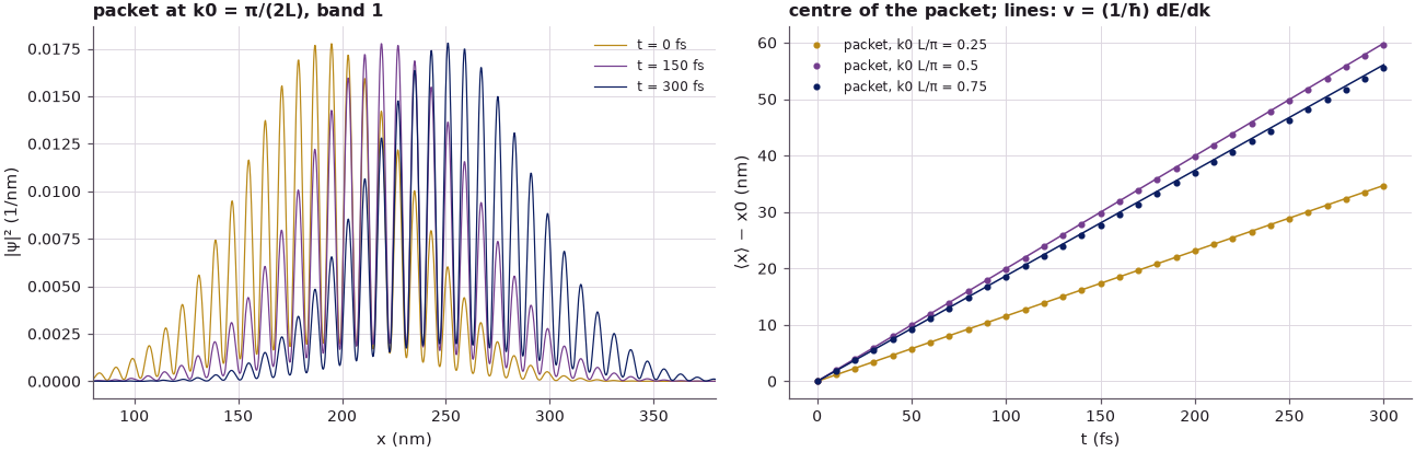
Figure computed by the notebook with open-nemo

The centre of the packet moves at constant speed, and the speed agrees with the slope of the band to within about 1 %. The small remaining difference comes from the packet itself: it contains a spread of wave numbers ($\Delta k \approx 1/(2\sigma) = 0.0125$ nm$^{-1}$), and the measured velocity is an average of $v(k)$ over that spread. The fastest packet is the one at $k_0 = \pi/(2L)$, near the inflection point of the band, where the slope is largest: 0.2 nm/fs, i.e. $2\times10^5$ m/s. In the left panel the carrier (the fast oscillation of the Bloch function inside each cell) is visible under the envelope, as on slide 3.

2. Velocity and effective mass across a band#

Newton's second law for the packet follows from two ingredients. A force $F$ does work $F\,dx = F v\,dt$ on the electron, which raises its band energy by $dE = (dE/dk)\,dk$; with $v = (1/\hbar)\,dE/dk$ this gives

\hbar\frac{dk}{dt} = F,

so $\hbar k$ plays the role of momentum (the crystal momentum). The acceleration is then

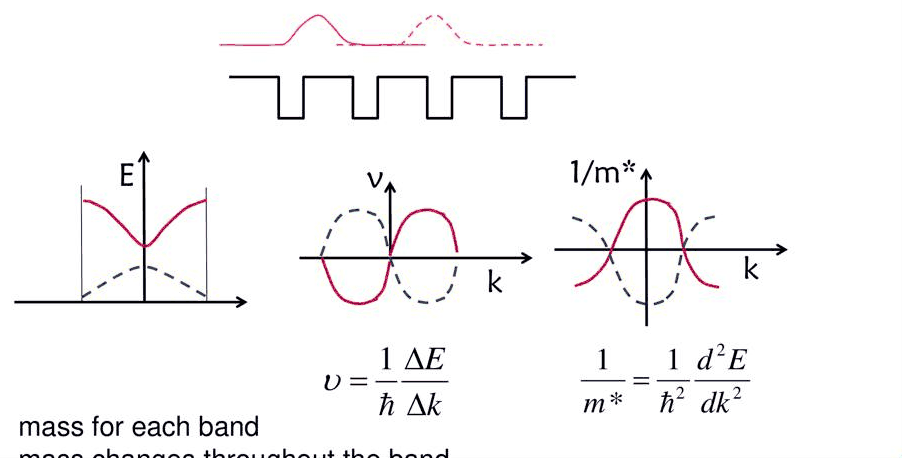
\frac{dv}{dt} = \frac{1}{\hbar}\frac{d^2E}{dk^2}\frac{dk}{dt} = \frac{1}{\hbar^2}\frac{d^2E}{dk^2}\,F \equiv \frac{F}{m^*}, \qquad \frac{1}{m^*} = \frac{1}{\hbar^2}\frac{d^2E}{dk^2}.

The effective mass $m^*$ is a property of the band at a given $k$, not the free electron mass. It changes through the band and changes sign: positive near the bottom of a band, infinite at the inflection point, negative near the top.

Slide 5: effective mass for a given band — Slide 5: $E(k)$, the velocity $v$ and the inverse mass $1/m^*$ for two bands (red and blue).

open-nemo's bands of the cell, now on the finer 0.05 nm grid used in Lectures 7.1 and 7.2, give $v(k)$ and $1/m^*(k)$ by numerical differentiation. At the band edges the mass also follows from the Kronig–Penney function $f(E)$ of Lecture 7.1: expanding $\cos kL = f(E)$ about an edge, where $f = \pm 1$, gives

\frac{m^*}{m_0} = \mp\,\frac{2}{L^2}\,\frac{\hbar^2}{2m_0}\,f'(E_\mathrm{edge}),

with the upper sign at $kL = 0$, where $f = \cos kL = +1$, and the lower sign at $kL = \pi$, where $f = -1$. $f'$ is the derivative of $f$ with respect to energy (1/eV).

Code50 lines · cell 5

from scipy.optimize import brentq


def kp_f(E, m=M, a=A, b=B, U=U0):
    al, be = np.sqrt(m * E / H2M0 + 0j), np.sqrt(m * (E - U) / H2M0 + 0j)
    return (
        np.cos(al * a) * np.cos(be * b) - (al**2 + be**2) / (2 * al * be) * np.sin(al * a) * np.sin(be * b)
    ).real


def kp_edge_mass(E_guess, sign, m=M, U=U0, de=1e-7):
    """Band edge near E_guess where f = sign (±1), and m*/m0 there from f'(E)."""
    e = brentq(lambda s: kp_f(s, m=m, U=U) - sign, E_guess - 0.01, E_guess + 0.01)
    fp = (kp_f(e + de, m=m, U=U) - kp_f(e - de, m=m, U=U)) / (2 * de)
    return e, -sign * 2 * H2M0 * fp / L**2


lead = cell_lead(0.05)
kq = np.linspace(-np.pi, np.pi, 2001)[:-1]  # k L, periodic grid (k L = −π is also +π)
Ek = lead.bands(kq)[:, :3]
h_k = (kq[1] - kq[0]) / L  # k step (1/nm)
up, dn = np.roll(Ek, -1, axis=0), np.roll(Ek, 1, axis=0)
v = (up - dn) / (2 * h_k) / HBAR  # nm/fs, central differences
inv_m = (up - 2 * Ek + dn) / h_k**2 / (2 * H2M0)  # m0/m* = (d²E/dk²) / (ħ²/m0)

print(" band  edge    E (eV)    m*/m0 open-nemo   m*/m0 Kronig–Penney")
i0, ipi = len(kq) // 2, 0
for j in range(3):
    for idx, name, sign in ((i0, "kL=0", 1), (ipi, "kL=π", -1)):  # f = cos kL = +1 or −1 there
        e_n = Ek[idx, j]
        e_kp, m_kp = kp_edge_mass(e_n, sign)
        print(f"  {j + 1}   {name}   {e_n:.4f}       {1 / inv_m[idx, j]:8.4f}          {m_kp:8.4f}")
jmax = np.argmax(v[i0:, 0]) + i0
print(
    f"band 1: largest velocity {v[jmax, 0]:.3f} nm/fs at kL/π = {kq[jmax] / np.pi:.3f}, "
    f"where m0/m* = {inv_m[jmax, 0]:.3f}"
)

fig, axes = plt.subplots(1, 3, figsize=(13, 4))
for j, c in zip(range(3), style.sweep(3)):
    axes[0].plot(kq / np.pi, Ek[:, j], color=c, label=f"band {j + 1}")
    axes[1].plot(kq / np.pi, v[:, j], color=c)
    axes[2].plot(kq / np.pi, inv_m[:, j], color=c)
axes[0].set(xlabel="k L / π", ylabel="E (eV)", title="bands (open-nemo)")
axes[1].set(xlabel="k L / π", ylabel="v (nm/fs)", title="group velocity (1/ħ) dE/dk")
axes[2].set(xlabel="k L / π", ylabel="m0 / m*", ylim=(-40, 40), title="inverse effective mass")
for ax in axes[1:]:
    ax.axhline(0, color=style.CONTEXT, lw=0.6)
axes[0].legend(frameon=False, fontsize=8)
fig.tight_layout();

 band  edge    E (eV)    m*/m0 open-nemo   m*/m0 Kronig–Penney
  1   kL=0   0.0617         0.0948            0.0948
  1   kL=π   0.0961        -0.0466           -0.0466
  2   kL=0   0.3822        -0.0086           -0.0086
  2   kL=π   0.2399         0.0208            0.0208
  3   kL=0   0.5286         0.0067            0.0067
  3   kL=π   0.8521        -0.0021           -0.0021
band 1: largest velocity 0.212 nm/fs at kL/π = 0.612, where m0/m* = -0.022

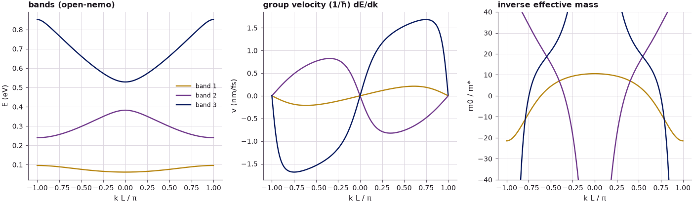
At the band edges open-nemo's curvature and the Kronig–Penney formula agree to the four digits printed. The first band has $m^* = 0.095\,m_0$ at its bottom, heavier than the GaAs mass $0.067\,m_0$ because the electron has to tunnel through the barriers to move, and $m^* = -0.047\,m_0$ at its top. The second band is lighter ($0.021\,m_0$ at its bottom, $-0.0086\,m_0$ at its top) and the third lighter still. Between the edges $1/m^*$ passes through zero, at the point where the velocity is largest (band 1: 0.212 nm/fs at $kL/\pi = 0.612$). There $m^*$ is infinite: a force changes $k$ but not the velocity. As the lecture puts it, there is a "mass for each band", and the "mass changes throughout the band"; a constant $m^*$ describes only the neighbourhood of a band edge.

3. A constant force: acceleration, negative mass and Bloch oscillations#

The lecture's next point (slide 6) is that the motion of a packet can be followed without the effective mass at all, by integrating the two equations of motion,

k(t) = k_0 + \int_0^t\frac{F}{\hbar}\,dt', \qquad x(t) = x_0 + \int_0^t v\big(k(t')\big)\,dt' .

For a uniform force the second integral has a closed form. With the potential energy $U(x) = F\,(x - x_m)$ (force $-F$, pointing to $-x$), $\hbar k$ decreases at the rate $F$ and the total energy $E(k) + U(x)$ is conserved, so

x(t) - x_0 = -\frac{E\big(k(t)\big) - E(k_0)}{F}, \qquad k(t) = k_0 - \frac{Ft}{\hbar}.

Because $E(k)$ is periodic, the packet does not run away: $k$ crosses the zone in the Bloch period $T_B = 2\pi\hbar/(FL)$, and $x$ swings back and forth over the band width divided by the force, $W/F$. The force is $F = 2$ meV/nm, which for an electron is an electric field of 2 mV/nm (20 kV/cm). Two packets start at the centre of the 80-cell chain, one at the bottom of the first band ($k_0 = 0$) and one at its top ($k_0 = \pi/L$), and are propagated with open-nemo's Hamiltonian plus $U(x)$.

Code46 lines · cell 7

F = 0.002  # force in eV/nm (2 meV per nm)
xm = 0.5 * NC * L
E_f, P_f = np.linalg.eigh(H + np.diag(F * (x - xm)))  # potential energy F (x − xm)
T_B = 2 * np.pi * HBAR / (F * L)
tB = np.linspace(0, T_B, 121)
band_p = lead_p.bands(np.linspace(-np.pi, np.pi, 2001))[:, 0]
W1 = band_p.max() - band_p.min()
e3 = lead_p.bands(np.array([-0.01, 0.0, 0.01]))[:, 0]
m_bot = 2 * H2M0 * (0.01 / L) ** 2 / (e3[0] - 2 * e3[1] + e3[2])  # m*/m0 at k = 0
print(
    f"Bloch period 2πħ/(FL) = {T_B:.1f} fs, band width W1 = {1e3 * W1:.1f} meV, "
    f"W1/F = {W1 / F:.2f} nm, m*/m0 at the band bottom = {m_bot:.4f}"
)

fig, ax = plt.subplots(figsize=(8.5, 4.2))
for k0L, c, lab in (
    (0.0, style.OPEN_NEMO, "start at k = 0 (bottom)"),
    (1.0, style.sweep(4)[3], "start at k = π/L (top)"),
):
    psi_t = evolve(packet(k0L * np.pi / L, xm, 40.0), tB, E_f, P_f)
    xc = (np.abs(psi_t) ** 2) @ x - xm
    kt = k0L * np.pi / L - F * tB / HBAR  # ħ dk/dt = −F
    pred = -(lead_p.bands(kt * L)[:, 0] - lead_p.bands(np.array([k0L * np.pi]))[0, 0]) / F
    ax.plot(tB, xc, "o", ms=3, color=c, label=f"packet, {lab}")
    ax.plot(tB, pred, "-", lw=1, color=c)
    print(
        f"{lab}: excursion {xc.min():+.2f} … {xc.max():+.2f} nm, "
        f"largest |packet − energy conservation| = {np.abs(xc - pred).max():.2f} nm"
    )
t_s = np.linspace(0, 0.3 * T_B, 50)
ax.plot(
    t_s,
    -0.5 * F * (2 * H2M0 / m_bot) / HBAR**2 * t_s**2,
    "--",
    color=style.CONTEXT,
    lw=1,
    label="−F t²/(2m*) with the band-bottom mass",
)
ax.set(
    xlabel="t (fs)",
    ylabel="⟨x⟩ − x0 (nm)",
    ylim=(-20, 20),
    title=f"uniform force F = {1e3 * F:.0f} meV/nm (pushes towards −x)",
)
ax.legend(frameon=False, fontsize=8, loc="lower left")
fig.tight_layout();

Bloch period 2πħ/(FL) = 258.5 fs, band width W1 = 34.5 meV, W1/F = 17.23 nm, m*/m0 at the band bottom = 0.0947
start at k = 0 (bottom): excursion -17.23 … +0.00 nm, largest |packet − energy conservation| = 0.07 nm
start at k = π/L (top): excursion -0.07 … +16.69 nm, largest |packet − energy conservation| = 0.54 nm

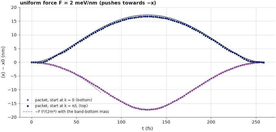
Started at the bottom of the band, the packet first accelerates in the direction of the force and follows $-Ft^2/(2m^*)$ with the band-bottom mass ($0.0947\,m_0$ on the 0.25 nm grid). As $k$ approaches $-\pi/L$ the mass turns negative and the packet slows down although the force keeps pushing; it stops at $-17.23$ nm $= -W_1/F$, returns, and is back at its start after one Bloch period, 258.5 fs. Started at the top of the band, where $m^* < 0$, the packet moves against the force, up to $+16.69$ nm: this is the negative mass of the lecture ("if you push it with a vector in one direction, it actually moves the other direction"). Both packets follow the energy-conservation prediction to within 0.07 and 0.54 nm, small compared with their width of 40 nm. Bloch oscillations are hard to see in bulk crystals, where $L$ is a fraction of a nanometre and $T_B$ is long compared with the time between scattering events; superlattices with periods of several nanometres, like this one, made them observable.

4. The effective mass is not essential: linear dispersion#

If $E(k)$ is linear, $E = \pm\hbar v_F|k|$, the velocity is defined everywhere (except exactly at the crossing) but $d^2E/dk^2$ is zero on both sides and undefined at the kink. "Mass appears to be ill-defined", yet the integral description of Section 3 works unchanged. Graphene is the example the lecture gives: near its Dirac points the bands are linear.

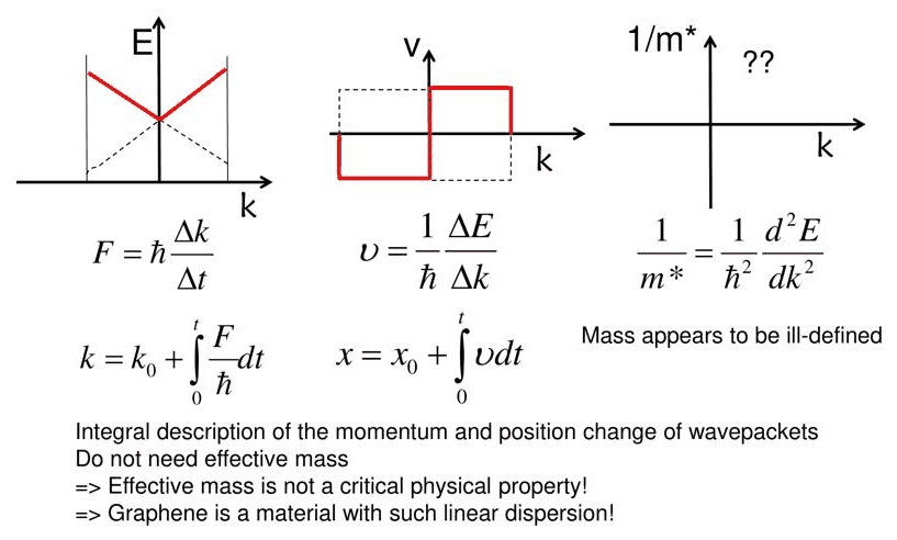
Slide 6: effective mass is not essential — Slide 6: a linear dispersion (left) has a well-defined velocity (centre) but no well-defined $1/m^*$ (right).

The smallest model with the same feature is a chain with two atoms per cell and alternating hopping energies $t_1$ (inside the cell) and $t_2$ (between cells), built as a nemo.Lead with $2\times2$ blocks. Its bands are $E = \pm|t_1 + t_2e^{ika}|$, with period $a$. For $t_1 \ne t_2$ a gap $2|t_1 - t_2|$ opens at $ka = \pi$, and expanding $E$ there gives the band-edge mass

m^* = \frac{\hbar^2|t_1 - t_2|}{t_1t_2a^2}.

For $t_1 = t_2$ the gap closes and the two bands cross linearly, the one-dimensional analogue of graphene's Dirac point (in graphene the two atoms per cell are the two sublattices). The parameters are graphene-like: $t_1 = 2.7$ eV and $a = 0.25$ nm.

Code35 lines · cell 9

a_c = 0.25  # chain period (nm)
t1 = 2.7  # intracell hopping (eV)
ka = np.linspace(0.6 * np.pi, np.pi, 4001)  # around the zone boundary k a = π
fig, (a1, a2) = plt.subplots(1, 2, figsize=(12, 4))
print(" t2/t1   gap (eV)   m*/m0 open-nemo   m*/m0 analytic   largest v (nm/fs)")
for r, c in zip((1.0, 0.9, 0.7), style.sweep(3)):
    t2 = r * t1
    chain2 = nemo.Lead(np.array([[0.0, -t1], [-t1, 0.0]]), np.array([[0.0, 0.0], [-t2, 0.0]]))
    E2 = chain2.bands(ka)[:, 1]  # upper band
    kk = ka / a_c
    v2 = np.gradient(E2, kk) / HBAR
    gap = 2 * abs(t1 - t2)
    if r < 1:
        curv = np.polyfit(kk[-10:] - np.pi / a_c, E2[-10:], 2)[0] * 2  # d²E/dk² at k a = π
        m_n, m_a = 2 * H2M0 / curv, 2 * H2M0 * abs(t1 - t2) / (t1 * t2 * a_c**2)
        print(
            f"  {r:.1f}     {gap:5.2f}        {m_n:.4f}           {m_a:.4f}            "
            f"{np.abs(v2).max():.3f}"
        )
    else:
        print(f"  {r:.1f}     {gap:5.2f}        undefined (kink)   0                 {np.abs(v2).max():.3f}")
    for s in (1, -1):
        a1.plot(s * (ka / np.pi - 1) + 1, E2, color=c, label=f"t2/t1 = {r}" if s == 1 else None)
        a1.plot(s * (ka / np.pi - 1) + 1, -E2, color=c)
    a2.plot(ka / np.pi, np.abs(v2), color=c, label=f"t2/t1 = {r}")
a1.set(
    xlabel="k a / π",
    ylabel="E (eV)",
    xlim=(0.6, 1.4),
    ylim=(-3, 3),
    title="two-band chain near the zone boundary",
)
a2.set(xlabel="k a / π", ylabel="|v| (nm/fs)", title="velocity of the upper band")
a1.legend(frameon=False, fontsize=8)
fig.tight_layout();

 t2/t1   gap (eV)   m*/m0 open-nemo   m*/m0 analytic   largest v (nm/fs)
  1.0      0.00        undefined (kink)   0                 1.026
  0.9      0.54        0.0502           0.0502            0.923
  0.7      1.62        0.1935           0.1935            0.718

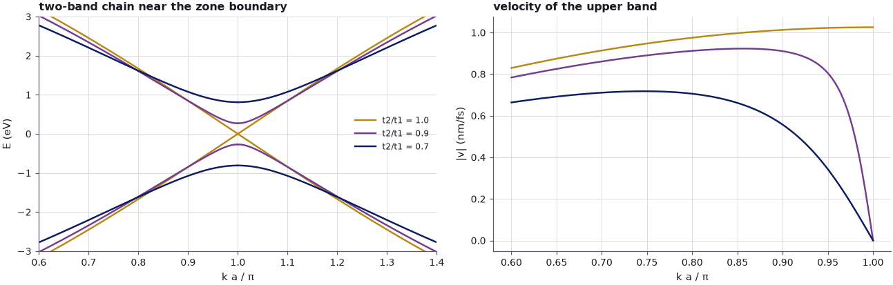
open-nemo's bands reproduce the analytic mass, and the mass shrinks in proportion to the gap: $0.0502\,m_0$ for a 0.54 eV gap, $0.194\,m_0$ for 1.62 eV. At $t_1 = t_2$ it would be zero, which only says that $d^2E/dk^2$ is infinite at the crossing. The velocity behaves smoothly throughout: its maximum grows only from 0.718 to 1.026 nm/fs, i.e. $1.03\times10^6$ m/s, close to the Fermi velocity of graphene. The same link between a small gap and a light mass is why narrow-gap semiconductors such as InAs and InSb have very light conduction-band masses. Velocity and band energies are the primary quantities; the effective mass is a convenient summary of them near a band edge.

5. Full bands carry no current; electrons and holes#

The current carried by the electrons in a ring of $N$ cells (length $NL$) is

I = -\frac{q}{NL}\sum_{i\,\in\,\text{filled}} v_i ,

with $q$ the elementary charge and $v_i$ the group velocity of state $i$. An empty band has no carriers and no current. In a full band every state with velocity $v(k)$ has a partner with $v(-k) = -v(k)$ (inversion symmetry, $E(k) = E(-k)$), and the Pauli principle puts exactly one electron (per spin) in each, so the sum is zero. A force shifts every $k$ by the same amount; a full band stays full and still carries nothing. Current needs a partially filled band, obtained by optical or thermal excitation or by doping.

Slide 9: electron and hole fluxes in partially filled bands — Slide 9: band 3 with a few electrons and band 2 with a few empty states, both shifted by a field $\mathcal{E}$; the current of the nearly full band 2 equals that of its empty states with positive charge (Shockley's parking-lot picture).

On a ring of 40 cells the velocities of all states of bands 1 and 2 follow from the Hellmann–Feynman expression of Section 1. Band 2 receives 7 electrons at its bottom ($kL = \pm\pi$), and band 1 loses the same 7 states at its top. Then every $k$ is moved by $-2\Delta k$, as a force acting for a short time would do.

Code41 lines · cell 11

Q = 1.602176634e-19  # elementary charge (C)
NR = 40  # cells in the ring
dk = 2 * np.pi / (NR * L)
n_all = np.arange(-NR // 2, NR // 2)


def velocities(band, shift=0.0):
    """Hellmann–Feynman velocities (nm/fs) of all ring states of `band`, every k moved by `shift`."""
    return np.array([bloch(lead_p, (n * dk + shift) * L, band)[2] for n in n_all])


def current_nA(v_sum):
    """I = −q Σ v / (N L), in nA (v in nm/fs = 10^6 m/s, N L in nm)."""
    return -Q * v_sum * 1e6 / (NR * L * 1e-9) * 1e9


v1, v2 = velocities(0), velocities(1)
v1s = velocities(0, shift=-0.37 * dk)
print(
    f"ring of {NR} cells, Δk = {dk:.4f} 1/nm; one electron at the fastest state carries "
    f"{abs(current_nA(v1.max())):.1f} nA"
)
print(f"band 1 full:                         I = {current_nA(v1.sum()):+.2e} nA")
print(f"band 1 full, all k moved by −0.37 Δk: I = {current_nA(v1s.sum()):+.2e} nA")

# band 2 nearly empty: 7 electrons at the bottom (k L = π), then all of them moved by −2 Δk
order2 = np.argsort(np.abs(np.abs(n_all * dk * L) - np.pi))  # the 7 states closest to k L = ±π
occ2 = np.zeros(NR, bool)
occ2[order2[:7]] = True
# band 1 nearly full: 7 empty states at the top (k L = π)
emp1 = np.zeros(NR, bool)
emp1[order2[:7]] = True
for shift_n in (0, -2):
    vs1, vs2 = velocities(0, shift_n * dk), velocities(1, shift_n * dk)
    I_e2 = current_nA(vs2[occ2].sum())
    I_filled1 = current_nA(vs1[~emp1].sum())
    I_holes1 = -current_nA(vs1[emp1].sum())  # +q for each empty state
    print(f"\nall k moved by {shift_n:+d} Δk:")
    print(f"  band 2, 7 electrons:      I = {I_e2:+8.2f} nA")
    print(f"  band 1, 33 electrons:     I = {I_filled1:+8.2f} nA   (sum over filled states)")
    print(f"  band 1, 7 holes (+q):     I = {I_holes1:+8.2f} nA   (sum over empty states)")

ring of 40 cells, Δk = 0.0196 1/nm; one electron at the fastest state carries 106.0 nA
band 1 full:                         I = +2.78e-14 nA
band 1 full, all k moved by −0.37 Δk: I = -5.21e-12 nA

all k moved by +0 Δk:
  band 2, 7 electrons:      I =    -0.00 nA
  band 1, 33 electrons:     I =    -0.00 nA   (sum over filled states)
  band 1, 7 holes (+q):     I =    -0.00 nA   (sum over empty states)

all k moved by -2 Δk:
  band 2, 7 electrons:      I =  +705.02 nA
  band 1, 33 electrons:     I =  +288.47 nA   (sum over filled states)
  band 1, 7 holes (+q):     I =  +288.47 nA   (sum over empty states)

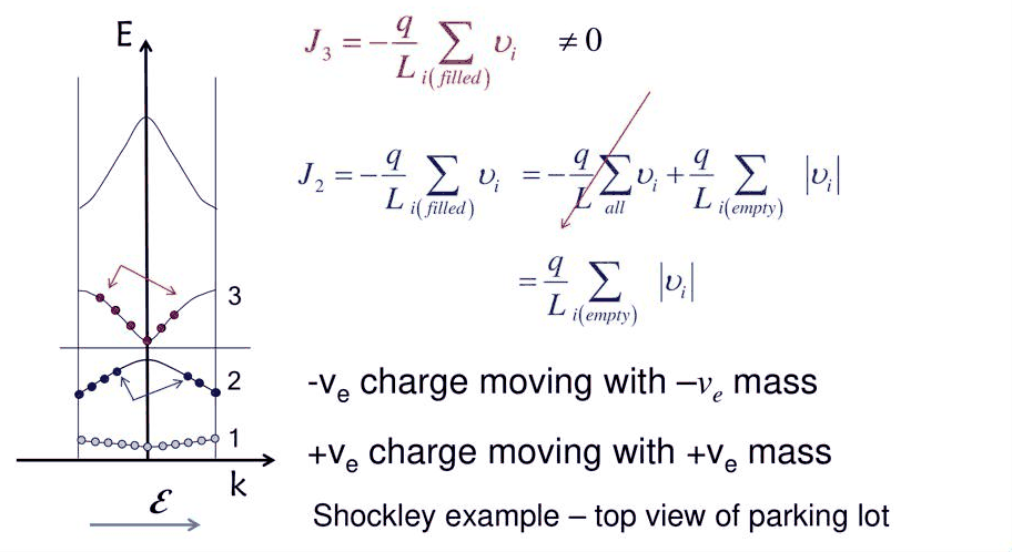
A full first band carries $3\cdot10^{-14}$ nA, and $-5\cdot10^{-12}$ nA after all its states are moved by an arbitrary fraction of $\Delta k$: zero to rounding, compared with the 106 nA of a single electron in the fastest state. Before the shift the partially filled bands carry nothing either, because their electrons are arranged symmetrically in $k$. After the shift by $-2\Delta k$ the 7 electrons of band 2 carry 705 nA, and the 33 electrons of band 1 carry 288.47 nA. The same 288.47 nA follows from the 7 empty states alone, counted with charge $+q$:

-\frac{q}{NL}\sum_{\text{filled}} v_i = -\frac{q}{NL}\Big(\sum_{\text{all}} v_i - \sum_{\text{empty}} v_i\Big) = +\frac{q}{NL}\sum_{\text{empty}} v_i ,

because the sum over all states vanishes. This is the hole: instead of 33 electrons with negative charge near the top of the band, where their mass is negative, one follows 7 empty states with positive charge and positive mass. Shockley's analogy is a two-storey parking garage: on the full lower floor no car can move, but if a few cars are lifted to the empty upper floor, both they and the gaps they leave behind can move. Both currents have the same sign: electrons in band 2 and holes in band 1 add up.

6. Exploration: electron and hole masses versus barrier height#

Electrons "fall" to the bottom of a band and holes "float" to its top, so the masses that matter for transport are those at the bottom of the conduction band and the top of the valence band. In the superlattice, band 1 plays the role of a valence band (holes at its top) and band 2 of a conduction band. The table follows the three band-edge masses as the barrier height $U_0$ is varied, from open-nemo's bands (a three-point curvature at the edge) and from the Kronig–Penney formula of Section 2.

Code15 lines · cell 13

print("  U0 (eV)   band-1 bottom m*/m0     band-1 top m*/m0      band-2 bottom m*/m0")
print("            open-nemo  K–P          open-nemo  K–P         open-nemo  K–P")
dq = 0.02
for U in (0.1, 0.2, 0.4, 0.6, 0.8):
    ld = cell_lead(0.05, U=U)
    row = []
    for kL0, j, sign in ((0.0, 0, 1), (np.pi, 0, -1), (np.pi, 1, -1)):
        e3 = ld.bands(np.array([kL0 - dq, kL0, kL0 + dq]))[:, j]
        m_n = 2 * H2M0 * (dq / L) ** 2 / (e3[0] - 2 * e3[1] + e3[2])
        m_kp = kp_edge_mass(e3[1], sign, U=U)[1]
        row += [m_n, m_kp]
    print(
        f"   {U:.1f}      {row[0]:.4f}  {row[1]:.4f}      {row[2]:+.4f}  {row[3]:+.4f}     "
        f"{row[4]:.4f}  {row[5]:.4f}"
    )

  U0 (eV)   band-1 bottom m*/m0     band-1 top m*/m0      band-2 bottom m*/m0
            open-nemo  K–P          open-nemo  K–P         open-nemo  K–P
   0.1      0.0691  0.0691      -0.0093  -0.0093     0.0073  0.0073
   0.2      0.0748  0.0748      -0.0201  -0.0200     0.0127  0.0127
   0.4      0.0948  0.0948      -0.0466  -0.0466     0.0208  0.0208
   0.6      0.1251  0.1252      -0.0808  -0.0808     0.0283  0.0283
   0.8      0.1659  0.1660      -0.1242  -0.1242     0.0368  0.0368

open-nemo and the Kronig–Penney formula agree to $10^{-4}\,m_0$ for every barrier height. Higher barriers make all three masses heavier, because the bands become narrower. For weak barriers the mass at the bottom of band 1 approaches the GaAs mass ($0.069\,m_0$ at 0.1 eV), while the masses on either side of the first gap, the top of band 1 ($-0.0093\,m_0$) and the bottom of band 2 ($0.0073\,m_0$), become very light: as in Section 4, a small gap means a light mass.

Summary#

A wave packet moves with the group velocity $v = (1/\hbar)\,dE/dk$; packets propagated in time with open-nemo's Hamiltonian move at the band's slope to within about 1 %.
A force changes the crystal momentum, $\hbar\,dk/dt = F$; the acceleration defines $1/m^* = (1/\hbar^2)\,d^2E/dk^2$, which depends on the band and on $k$, is infinite at the band's inflection point and negative near its top.
Under a constant force a packet performs a Bloch oscillation of amplitude $W/F$ and period $2\pi\hbar/(FL)$; started at the band top it moves against the force.
The effective mass is not fundamental: for a linear dispersion it is undefined, and it shrinks with the gap, while velocities stay finite.
Empty and full bands carry no current. A nearly full band is described by its empty states, holes with positive charge and positive mass.

Exercises#

Propagate a packet in band 2 (packet(..., band=1)) with $k_0 = \pi/(2L)$. In which direction does it move, and why?
Repeat Section 3 with $F = 1$ and $4$ meV/nm. Check that $T_B \propto 1/F$ and that the amplitude is $W_1/F$.
In Section 4, compute $m^*$ for $t_2/t_1 = 0.95$ and $0.99$ and plot $m^*$ against the gap.
In Section 5, shift the 7 electrons of band 2 by $+2\Delta k$ instead of $-2\Delta k$. What happens to the currents of band 1 and band 2?