

Lecture 10.3
Introduction to transport — coherent tunneling in a double barrier and the Landauer picture
In the lecture
- the exact transmission of a double barrier in Fabry–Pérot form, built from the transmission and reflection of each barrier and the round-trip phase in the well
- the resonance condition \(\theta(E) = 2n\pi\) (a closed, quantized orbit) and its particle-in-a-box limit for huge barriers; penetration into the barriers lowers the resonance
- the round-trip phase and the time an electron lingers in the well (Wigner dwell time)
- a numerical example (5 nm | 5 nm | 5 nm GaAs/AlGaAs): a sharp and a broad resonance, and where in energy the flux flows (the running integral of \(T\))
- the Breit–Wigner (Lorentzian) approximation and its delta-function limit; good for the sharp peak, poor for the tails of broad states
- the Landauer current in two corner cases, low temperature and narrow resonances, both giving \(I = (2e/\hbar)\,\Gamma_L\Gamma_R/(\Gamma_L + \Gamma_R)\) — the rate-equation result of Lecture 10.2
In this notebook
you implement the Fabry–Pérot formula and compare it with open-nemo's
open-boundary transmission, follow the lowest resonance to the particle-in-a-box limit, relate the
phase derivative to the round-trip time and the escape rates, reproduce the lecture's running
integral and Breit–Wigner comparison, and evaluate the two Landauer corner cases with
nemo.landauer_current.
Run it on your own machine
The notebook needs open-nemo (Python ≥ 3.10 and a C++20 compiler; BLAS/LAPACK).
git clone https://github.com/denphi/open-nemo.git && cd open-nemo
python3 -m venv .venv && source .venv/bin/activate
pip install -e ".[notebooks]"
jupyter lab From_Atoms_to_Devices/05_introduction_to_transport/10_3_coherent_tunneling_and_landauer.ipynbCode
import numpy as np
import matplotlib.pyplot as plt
from scipy.integrate import cumulative_trapezoid
from scipy.optimize import brentq
from scipy.signal import find_peaks, peak_widths
import opennemo as nemo
from opennemo.visualization import style
from opennemo.structures.statistics import fermi

style.use(notebook=True)
H2M0 = nemo.core.units.HBAR2_2M0          # ħ²/2m₀ = 0.0381 eV nm²
HBAR, Q, KB = nemo.core.units.HBAR, nemo.core.units.Q, nemo.core.units.KB
EM = nemo.structures.materials.EffectiveMassMaterial
1. The exact transmission in Fabry–Pérot form#
In Section 6 the double barrier was solved with one scattering matrix per interface. Klimeck now writes the answer in a form that shows the physics. Treat each barrier as a standalone scatterer with transmission \(T_{L,R}(E)\) and reflection \(R_{L,R} = 1 - T_{L,R}\). An electron in the well bounces back and forth; each round trip adds the phase
with \(k = \sqrt{2m^*E}/\hbar\) the wave vector in the well (and the leads), \(w\) the well width and \(\phi_{L,R}\) the phases of the reflection amplitudes of the two barriers seen from inside the well. Summing the multiply reflected waves gives the Fabry–Pérot form
The left and right sections stay uncoupled, so the form remains exact for unequal barriers and under bias. The transmission peaks where \(\cos\theta = 1\), \(\theta(E) = 2n\pi\): the wave returns in phase after a round trip, a closed quantized orbit. For a symmetric structure the peak is then \(T_L^2/(1 - R_L)^2 = 1\).
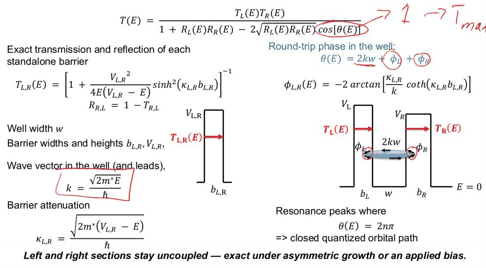
The slide gives the single-barrier quantities for one effective mass, \(T_{L,R} = [1 + V^2\sinh^2(\kappa b)/4E(V - E)]^{-1}\) and \(\phi = -2\arctan[(\kappa/k)\coth(\kappa b)]\), with \(\kappa = \sqrt{2m^*(V - E)}/\hbar\) the attenuation in a barrier of height \(V\) and thickness \(b\). The lecture's example has different masses in the well (\(0.067\,m_0\)) and in the barriers (\(0.092\,m_0\)). Then the matching condition at each interface is continuity of \(\psi\) and of \(\psi'/m\) (BenDaniel–Duke), and \(k\) and \(\kappa\) are replaced by \(\tilde k = k/m_w\) and \(\tilde\kappa = \kappa/m_b\) in the ratios:
For equal masses the first expression is the slide's. The code below computes the reflection amplitude \(r\) of one barrier exactly, by matching plane waves at its two interfaces, so that \(\phi = \arg r\), and compares the Fabry–Pérot \(T(E)\) with open-nemo's transmission of the discretized structure (10 nm GaAs leads, 0.025 nm grid).
Code
MW, MB, V0, W, B = 0.067, 0.092, 0.3, 5.0, 5.0     # masses (m0), barrier height (eV), widths (nm)


def barrier(E, b=B, v=V0, mb=MB):
    # exact r and t of one barrier (thickness b) between GaAs regions; psi and psi'/m continuous
    k = np.sqrt(MW * E / H2M0 + 0j)
    q = np.sqrt(mb * (E - v) / H2M0 + 0j)                 # q = i κ below the barrier top
    s = (k / MW) / (q / mb)
    a, c = 0.5 * (1 + s) * np.exp(-1j * q * b), 0.5 * (1 - s) * np.exp(1j * q * b)
    one_plus_r, one_minus_r = a + c, (a - c) / s           # per unit transmitted amplitude
    incident = 0.5 * (one_plus_r + one_minus_r)
    return 0.5 * (one_plus_r - one_minus_r) / incident, 1 / incident


def theta(E, w=W, bl=B, br=B, v=V0, mb=MB):
    k = np.sqrt(MW * E / H2M0)
    return 2 * k * w + np.angle(barrier(E, bl, v, mb)[0]) + np.angle(barrier(E, br, v, mb)[0])


def fabry_perot(E, w=W, bl=B, br=B, v=V0, mb=MB):
    (rl, tl), (rr, tr) = barrier(E, bl, v, mb), barrier(E, br, v, mb)
    RL, RR = abs(rl) ** 2, abs(rr) ** 2
    th = theta(E, w, bl, br, v, mb)
    return abs(tl) ** 2 * abs(tr) ** 2 / (1 + RL * RR - 2 * np.sqrt(RL * RR) * np.cos(th))


def slide_formulas(E, b=B, v=V0, mb=MB):
    # single-barrier T and phase of the slide, with k/m_w and κ/m_b in the ratios (E < v)
    k, kap = np.sqrt(MW * E / H2M0), np.sqrt(mb * (v - E) / H2M0)
    kt, qt = k / MW, kap / mb
    t1 = 1 / (1 + ((kt**2 + qt**2) / (2 * kt * qt)) ** 2 * np.sinh(kap * b) ** 2)
    return t1, -2 * np.arctan(qt / kt / np.tanh(kap * b))


gaas = EM("GaAs", MW, 12.9)
algaas = EM("AlGaAs", MB, 12.2, conduction_band_edge=V0)


def double_barrier(bl=B, w=W, br=B, dx=0.025, barrier_material=algaas):
    mats = (gaas, barrier_material, gaas, barrier_material, gaas)
    return nemo.Heterostructure1D([nemo.Layer(m, d) for m, d in zip(mats, (10, bl, w, br, 10))], spacing=dx)


dev = double_barrier()
tr = nemo.Transport(dev.hamiltonian)
E = np.linspace(0.001, 0.45, 3000)
T_nemo, T_fp = tr.transmission(E), fabry_perot(E)
r, t = barrier(E)
print(f"largest |ln(T open-nemo / T Fabry-Pérot)| = {np.abs(np.log(T_nemo / T_fp)).max():.3f}")
print(f"largest |R + T - 1| of one barrier = {np.abs(abs(r)**2 + abs(t)**2 - 1).max():.1e}")
for e in (0.05, 0.08, 0.2):
    t1, ph = slide_formulas(e)
    print(f"E = {e:4.2f} eV: T_1 exact {abs(barrier(e)[1])**2:.4e}, slide {t1:.4e};"
          f"  φ exact {np.angle(barrier(e)[0]):+.4f}, slide {ph:+.4f} rad")
largest |ln(T open-nemo / T Fabry-Pérot)| = 0.042
largest |R + T - 1| of one barrier = 1.0e-15
E = 0.05 eV: T_1 exact 1.1419e-03, slide 1.1419e-03;  φ exact -2.1758, slide -2.1769 rad
E = 0.08 eV: T_1 exact 2.4258e-03, slide 2.4258e-03;  φ exact -1.9108, slide -1.9126 rad
E = 0.20 eV: T_1 exact 2.2800e-02, slide 2.2800e-02;  φ exact -1.0919, slide -1.0989 rad
The Fabry–Pérot formula and open-nemo agree to within about 4 % everywhere, over twelve decades of \(T\); the remaining difference is the discretization of the 0.025 nm grid. The generalized single-barrier transmission is exact. The slide's phase formula is the thick-barrier form (exact when \(\coth\kappa b = 1\)): it differs from the exact \(\arg r\) by \(1\)–\(2\cdot10^{-3}\) rad near the lower resonance and by \(7\cdot10^{-3}\) rad at 0.2 eV. Below, the resonances are located on a fine grid with all three methods.
Code
def slide_T(E):
    t1, ph = slide_formulas(E)
    th = 2 * np.sqrt(MW * E / H2M0) * W + 2 * ph
    return t1**2 / (1 + (1 - t1) ** 2 - 2 * (1 - t1) * np.cos(th))


res = nemo.resonances(dev)
print("  open-nemo resonance (meV)   Γ (meV)   peak of T: open-nemo   Fabry-Pérot   slide phase")
for e0, g in zip(res["energy"], res["width"]):
    Ef = e0 + np.linspace(-8, 8, 40001) * max(g, 5e-4)
    peaks = [Ef[np.argmax(f(Ef))] * 1e3 for f in (tr.transmission, fabry_perot)]
    slide = Ef[np.argmax(slide_T(Ef))] * 1e3 if e0 < V0 - 0.02 else np.nan
    print(f"        {e0 * 1e3:8.3f}            {g * 1e3:7.4f}       {peaks[0]:8.3f}"
          f"          {peaks[1]:8.3f}       {slide:8.3f}")

fig, axes = plt.subplots(1, 2, figsize=(10.5, 4), gridspec_kw={"width_ratios": [0.8, 1]})
axes[0].plot(dev.x - 10, dev.band_edge, color=style.OPEN_NEMO)
for e0 in res["energy"]:
    axes[0].axhline(e0, color=style.CONTEXT, ls="--", lw=0.8)
axes[0].set(xlabel="z (nm)", ylabel="E (eV)", title="5 nm | 5 nm | 5 nm, 0.3 eV")
axes[1].semilogx(T_nemo, E, color=style.OPEN_NEMO, lw=1.3, label="open-nemo")
axes[1].semilogx(T_fp, E, ":", color=style.REFERENCE, label="Fabry–Pérot")
axes[1].set(xlabel="T(E)", ylabel="E (eV)", xlim=(1e-12, 3), title="exact transmission")
axes[1].legend(frameon=False, fontsize=8)
fig.tight_layout()
  open-nemo resonance (meV)   Γ (meV)   peak of T: open-nemo   Fabry-Pérot   slide phase
          81.801             0.1293         81.801            81.804         81.894
         292.010             8.9928        292.402           292.409            nan

The exact phase puts the lower peak at 81.804 meV, open-nemo at 81.801 meV. The slide's phase formula shifts it to 81.894 meV: a phase error of a few \(10^{-3}\) rad moves this resonance by 70 % of its width. The lecture's slide 13 (below) reports the two resonances at 81.80 and 292.41 meV, matching the computed transmission peaks (81.80 and 292.40 meV; the real part of open-nemo's eigenvalue for the broad upper state is 292.01 meV). Its widths differ: 0.14 meV for the lower and 4.96 meV for the upper resonance. open-nemo's complex eigenvalue gives 0.129 meV for the lower one, within 8 %. For the upper one, which sits at the barrier top and is far from a Lorentzian, the computed width is 8.99 meV (the full width at half maximum of \(T(E)\) is computed in Section 4); the lecture does not say how its value was extracted.
2. Huge barriers: the particle in a box#
For identical huge barriers the electron cannot enter them. A hard wall reflects with \(r = -1\), a phase of \(\pm\pi\) per wall; the two walls add \(\pm 2\pi\) to the round trip, which the condition \(\theta = 2n\pi\) cannot distinguish from no phase at all (this is the slide's "\(\phi_{L,R} \to 0\)"). The resonance condition becomes \(2kw = 2n\pi\), the particle in a box:
For \(w = 5\) nm and \(m^* = 0.067\,m_0\) the ground state would be at 224.5 meV, almost three times the computed 81.8 meV. The wave function penetrates into the barriers; the phases \(\phi_{L,R}\) make the round trip longer, as if the well were wider, and the resonance lower. The limit needs a large \(\kappa\), that is tall barriers. Thick barriers alone only make \(\coth(\kappa b) \to 1\): the resonance then approaches the bound state of a finite well, found from \(\theta(E) = 0\) with \(\phi = -2\arctan(\tilde\kappa/\tilde k)\), equivalently \(\tilde k\tan(kw/2) = \tilde\kappa\).
Code
def finite_well(v, mb=MB):
    # ground state of a finite well (BenDaniel-Duke): (k/m_w) tan(k w/2) = κ/m_b
    def f(e):
        k, kap = np.sqrt(MW * e / H2M0), np.sqrt(mb * (v - e) / H2M0)
        return (k / MW) * np.sin(k * W / 2) - (kap / mb) * np.cos(k * W / 2)
    return brentq(f, 1e-6, min(v, H2M0 * np.pi**2 / MW / W**2) - 1e-9)


e_box = H2M0 * np.pi**2 / MW / W**2
print(f"particle in a box, w = {W} nm: E1 = {e_box * 1e3:.1f} meV")
print("\ntaller barriers (b = 5 nm)")
print("  V (eV)   E1 open-nemo (meV)   E1 finite well (meV)   effective width (nm)")
for v in (0.3, 1.0, 3.0, 10.0, 100.0):
    e_fw = finite_well(v)
    tall = EM("tall barrier", MB, 12.2, conduction_band_edge=v)
    e_nemo = nemo.resonances(double_barrier(barrier_material=tall))["energy"][0] if v <= 10 else np.nan
    print(f"  {v:6.1f}        {e_nemo * 1e3:8.2f}             {e_fw * 1e3:8.2f}"
          f"              {np.pi / np.sqrt(MW * e_fw / H2M0):6.2f}")
print("\nthicker barriers (V = 0.3 eV)")
print("  b (nm)   E1 (meV)   Γ (meV)")
for b in (2, 3, 5, 7, 9):
    r_b = nemo.resonances(double_barrier(bl=b, br=b, dx=0.05))
    print(f"   {b:4.1f}     {r_b['energy'][0] * 1e3:7.3f}   {r_b['width'][0] * 1e3:.2e}")
print(f"finite well, V = 0.3 eV: E1 = {finite_well(V0) * 1e3:.3f} meV")
particle in a box, w = 5.0 nm: E1 = 224.5 meV

taller barriers (b = 5 nm)
  V (eV)   E1 open-nemo (meV)   E1 finite well (meV)   effective width (nm)
     0.3           81.80                81.83                8.28
     1.0          122.14               122.16                6.78
     3.0          154.69               154.72                6.02
    10.0          181.53               181.60                5.56
   100.0             nan               209.43                5.18

thicker barriers (V = 0.3 eV)
  b (nm)   E1 (meV)   Γ (meV)
    2.0      79.632   9.78e+00
    3.0      81.386   2.34e+00
    5.0      81.793   1.29e-01
    7.0      81.813   7.09e-03
    9.0      81.814   3.89e-04
finite well, V = 0.3 eV: E1 = 81.826 meV
With taller barriers the lowest resonance climbs from 81.8 meV towards the box value: 122.1 meV at 1 eV, 181.5 meV at 10 eV, and 209.4 meV (finite well) at an unphysical 100 eV. open-nemo and the finite well agree to within 0.07 meV. The effective width \(w_\mathrm{eff} = \pi/k\), the box that has the same ground state, shrinks from 8.28 nm to 5.18 nm. Thicker barriers instead leave the energy at the finite-well value (81.814 meV on the 0.05 nm grid, 81.826 meV analytically) and only make the resonance sharper, by a factor of 18 per 2 nm of barrier.
3. Round-trip phase and dwell time#
A longer round-trip phase means a longer time in the well. Klimeck defines the Wigner dwell time as the energy derivative of the accumulated phase,
and states that near a quasi-bound state \(\tau_D = \hbar/(\Gamma_L + \Gamma_R)\), with \(\Gamma_{L,R}\) the escape rates through each barrier in energy units.

The two statements describe different times, and it is instructive to compute both. The derivative of the round-trip phase itself, \(\hbar\,d\theta/dE\), is the time of one round trip: the classical time \(2w_\mathrm{eff}/v\) with \(v = \hbar k/m^*\). On each round trip the electron escapes with probability \(T_L + T_R\), so it makes about \(1/(T_L + T_R)\) round trips before it leaves, and
This is the lifetime of the quasi-bound state. The fast phase sweep of the slide is the phase of the transmission amplitude \(t(E)\), the sum of all round trips: it changes by \(\pi\) across the resonance, and its derivative at the peak is \(2/(\Gamma_L + \Gamma_R)\).
Code
def t_total(E, w=W):
    # transmission amplitude of the double barrier (sum over round trips), up to a constant phase
    (rl, tl), (rr, tr_) = barrier(E), barrier(E)
    k = np.sqrt(MW * E / H2M0)
    return tl * tr_ * np.exp(1j * k * w) / (1 - rl * rr * np.exp(2j * k * w))


h = 1e-7
print(" E_r (meV)   ħ dθ/dE (fs)   2w_eff/v (fs)   T_L = T_R   Γ_L = T_L/(dθ/dE) (meV)"
      "   Γ_L + Γ_R (meV)   ħ/(Γ_L + Γ_R) (ps)   Γ open-nemo (meV)")
for e0, g in zip(res["energy"], res["width"]):
    dth = (theta(e0 + h) - theta(e0 - h)) / (2 * h)
    k = np.sqrt(MW * e0 / H2M0)
    v = 2 * H2M0 * k / (MW * HBAR)                    # group velocity ħk/m* in nm/s
    w_eff = np.pi / k if e0 < 0.2 else np.nan         # box with the same ground state
    t1 = abs(barrier(e0)[1]) ** 2
    g_lr = 2 * t1 / dth
    print(f"  {e0 * 1e3:7.2f}      {HBAR * dth * 1e15:6.1f}          {2 * w_eff / v * 1e15:6.1f}"
          f"         {t1:.2e}          {t1 / dth * 1e3:.4f}               {g_lr * 1e3:.4f}"
          f"            {HBAR / g_lr * 1e12:7.3f}            {g * 1e3:.4f}")
e0, g = res["energy"][0], res["width"][0]
arg_t = np.unwrap(np.angle(t_total(e0 + g * np.linspace(-20, 20, 4001))))
slope = (np.angle(t_total(e0 + h) / t_total(e0 - h))) / (2 * h)
print(f"\nphase of t: changes by {(arg_t[-1] - arg_t[0]) / np.pi:.3f} π across ±20Γ;"
      f" d arg t/dE at the peak = {slope:.0f} /eV, 2/Γ = {2 / g:.0f} /eV")
 E_r (meV)   ħ dθ/dE (fs)   2w_eff/v (fs)   T_L = T_R   Γ_L = T_L/(dθ/dE) (meV)   Γ_L + Γ_R (meV)   ħ/(Γ_L + Γ_R) (ps)   Γ open-nemo (meV)
    81.80        25.7            25.3         2.52e-03          0.0646               0.1291              5.098            0.1293
   292.01        18.7             nan         1.19e-01          4.2046               8.4092              0.078            8.9928

phase of t: changes by 0.997 π across ±20Γ; d arg t/dE at the peak = 15445 /eV, 2/Γ = 15472 /eV
For the lower resonance one round trip takes 25.7 fs, close to the classical time of 25.3 fs for the effective width of 8.28 nm; the round-trip time of the upper resonance is 18.7 fs (it sits at the barrier top, where \(w_\mathrm{eff}\) is not defined). Each barrier transmits \(2.5\cdot10^{-3}\) of the flux at the lower resonance, so the electron makes about 200 round trips before it escapes: the escape rate through one barrier is \(\Gamma_L = 0.0646\) meV, \(\Gamma_L + \Gamma_R = 0.1291\) meV agrees with the open-system eigenvalue (0.1293 meV) and with the one-sided widths of Lecture 10.2, and the lifetime is \(\hbar/(\Gamma_L + \Gamma_R) = 5.10\) ps. For the upper resonance the estimate (8.41 meV against 8.99 meV) is cruder, because the barriers are no longer good reflectors. The phase of \(t\) sweeps by \(0.997\pi\) across the lower resonance, at the rate 15445 /eV at the peak, against \(2/\Gamma = 15472\) /eV.
4. The numerical example: where does the flux flow?#
For transport the question is where in energy the electrons can flow. Klimeck plots, next to \(T(E)\), the running integral \(\int_0^E T(E')\,dE'\), the cumulative spectral content. A sharp resonance gives a sharp step (flux in a narrow energy range); a broad resonance gives a broad ramp (flux spread over a wide range), and a much larger total.

The energy grid below is uniform with dense patches of \(\pm 40\,\Gamma\) around each resonance, so that the 0.13 meV peak is resolved.
Code
patches = [e0 + g * np.linspace(-40, 40, 4001) for e0, g in zip(res["energy"], res["width"])]
Ec = np.unique(np.concatenate([np.linspace(1e-4, 0.45, 9000)] + patches))
Ec = Ec[(Ec > 0) & (Ec <= 0.45)]
Tc = tr.transmission(Ec)
cum = cumulative_trapezoid(Tc, Ec, initial=0) * 1e3                         # meV
for i in find_peaks(Tc, prominence=0.3)[0]:
    w_half = peak_widths(Tc, [i], rel_height=0.5)[0][0]
    idx = np.arange(len(Ec))
    fwhm = np.interp(i + w_half / 2, idx, Ec) - np.interp(i - w_half / 2, idx, Ec)
    print(f"peak at {Ec[i] * 1e3:7.2f} meV: T = {Tc[i]:.4f}, FWHM of T(E) = {fwhm * 1e3:.3f} meV")
for e in (0.07, 0.09, 0.25, 0.30, 0.35, 0.45):
    print(f"∫_0^E T dE' up to {e * 1e3:3.0f} meV: {np.interp(e, Ec, cum):8.4f} meV")
print(f"π Γ_1 / 2 = {np.pi * res['width'][0] / 2 * 1e3:.4f} meV")
peak at   81.80 meV: T = 1.0000, FWHM of T(E) = 0.129 meV
peak at  292.42 meV: T = 1.0000, FWHM of T(E) = 8.533 meV
∫_0^E T dE' up to  70 meV:   0.0001 meV
∫_0^E T dE' up to  90 meV:   0.2024 meV
∫_0^E T dE' up to 250 meV:   0.2453 meV
∫_0^E T dE' up to 300 meV:  10.7577 meV
∫_0^E T dE' up to 350 meV:  15.5656 meV
∫_0^E T dE' up to 450 meV:  60.2391 meV
π Γ_1 / 2 = 0.2031 meV
The lower peak has a full width at half maximum of 0.129 meV, equal to the eigenvalue width; the upper peak, at 292.42 meV, is 8.53 meV wide and asymmetric, as the transmission stays high above the barrier top. The running integral jumps by 0.2024 meV at the lower resonance — the area \(\pi\Gamma/2 = 0.2031\) meV of a unit-height Lorentzian — and then rises by 10.5 meV between 250 and 300 meV, across the upper resonance: about 50 times more flux, spread over a range about 70 times wider.
5. The Breit–Wigner (Lorentzian) approximation#
Near an isolated resonance the Fabry–Pérot form becomes a Lorentzian, the Breit–Wigner formula:
Only symmetric structures (\(\Gamma_L = \Gamma_R\)) reach \(T = 1\); any asymmetry lowers the peak. The total spectral content is \(\pi\Gamma\) for a symmetric structure (with \(\Gamma = \Gamma_L = \Gamma_R\)), so broad resonances carry large flow; for \(\Gamma_\mathrm{small} \ll \Gamma_\mathrm{large}\) it is \(\approx 2\pi\Gamma_\mathrm{small}\): the highest or widest barrier limits the flow. If the resonance is narrow compared with every other variation in energy, the Lorentzian can be replaced by a delta function of the same weight, \(T_\delta(E) = 2\pi\,\Gamma_L\Gamma_R/(\Gamma_L + \Gamma_R)\,\delta(E - E_r)\).
The lecture compares the exact \(T(E)\) with Lorentzians built from the extracted widths. Here
\(\Gamma_L = \Gamma_R = \Gamma/2\) with \(\Gamma\) from nemo.resonances.
Code
def t_bw(E, e0, gl, gr):
    return gl * gr / ((E - e0) ** 2 + ((gl + gr) / 2) ** 2)


bw1 = t_bw(Ec, res["energy"][0], res["width"][0] / 2, res["width"][0] / 2)
bw2 = t_bw(Ec, res["energy"][1], res["width"][1] / 2, res["width"][1] / 2)
cum1 = cumulative_trapezoid(bw1, Ec, initial=0) * 1e3
cum12 = cumulative_trapezoid(bw1 + bw2, Ec, initial=0) * 1e3
print("    E (meV)   ∫T exact (meV)   ∫T_BW1 (meV)   ∫(T_BW1 + T_BW2) (meV)   (BW1+BW2)/exact")
for e in (0.0815, 0.09, 0.15, 0.25, 0.30, 0.45):
    a, b1, b12 = (np.interp(e, Ec, c) for c in (cum, cum1, cum12))
    print(f"   {e * 1e3:7.1f}       {a:8.4f}        {b1:8.4f}          {b12:8.4f}             {b12 / a:6.3f}")

fig, axes = plt.subplots(1, 3, figsize=(13, 4.2))
for ax, lo, hi in ((axes[0], 0.0812, 0.0824), (axes[1], 0.0, 0.45)):
    ax.semilogx(Tc, Ec, color=style.OPEN_NEMO, lw=1.4, label="exact (open-nemo)")
    ax.semilogx(bw1, Ec, "--", color=style.REFERENCE, lw=1, label="T_BW1")
    ax.semilogx(bw2, Ec, ":", color=style.CONTEXT, lw=1.2, label="T_BW2")
    ax.set(xlabel="T(E)", ylabel="E (eV)", ylim=(lo, hi), xlim=(1e-10 if hi > 0.1 else 1e-3, 3))
axes[0].set_title("lower resonance (zoom)")
axes[1].set_title("both resonances")
axes[1].legend(frameon=False, fontsize=8, loc="lower left")
axes[2].semilogx(cum, Ec, color=style.OPEN_NEMO, lw=1.4, label="∫ T exact")
axes[2].semilogx(cum12, Ec, "--", color=style.REFERENCE, lw=1, label="∫ (T_BW1 + T_BW2)")
axes[2].set(xlabel="∫₀ᴱ T dE' (meV)", ylabel="E (eV)", xlim=(1e-6, 30), title="running integral")
axes[2].legend(frameon=False, fontsize=8, loc="upper left")
fig.tight_layout()
    E (meV)   ∫T exact (meV)   ∫T_BW1 (meV)   ∫(T_BW1 + T_BW2) (meV)   (BW1+BW2)/exact
      81.5         0.0127          0.0136            0.0404              3.179
      90.0         0.2024          0.2025            0.2333              1.153
     150.0         0.2039          0.2029            0.2760              1.353
     250.0         0.2453          0.2030            0.6132              2.500
     300.0        10.7577          0.2030           11.9548              1.111
     450.0        60.2391          0.2030           14.1317              0.235

The lower Lorentzian fits the exact peak, and its running integral reproduces the step, 0.2025 meV at 90 meV against 0.2024 meV exact, "even on a log scale". The upper Lorentzian fits its peak, but its tails are far too wide: at 90 meV, just above the lower resonance, the tail of \(T_{BW2}\) already adds 0.031 meV to the running integral (15 % of the step), and at 250 meV the sum of the two Lorentzians is 2.5 times the exact integral. Klimeck estimates the effect of the tails as "something like 10, 20%" of the integral. Above the barrier top the opposite happens: the exact transmission stays close to one while the Lorentzian decays, and at 450 meV the Lorentzians carry only 24 % of the exact flux. This is the lecture's observation that the tail of \(T_{BW2}\) contributes to the flux in the range of \(T_{BW1}\). Klimeck's verdict: the Lorentzian fits peaks well, but it is not a good approximation to broad states in quantum wells.

6. Landauer transport in two corner cases#
The current through the structure is the Landauer integral
Cold temperatures and high bias. At \(T = 0\) the Fermi functions are steps. If the resonance lies in the window, \(f_L(E_r) = 1\) and \(f_R(E_r) = 0\), and if \(\Gamma_{L,R} \ll eV\) the integral over the window takes in the whole Lorentzian:
Narrow resonances. At finite temperature, if \(\Gamma_{L,R} \ll k_BT\), the Fermi functions do not change across the resonance and the delta function gives
The lecture's example has \(\Gamma = 0.14\) meV and \(k_BT = 26\) meV at 300 K, a ratio of 0.00538. Both are the rate-equation current of Lecture 10.2. As in the lecture, the transmission is that of the unbiased structure; only the Fermi levels move.

Code
e0, g = res["energy"][0], res["width"][0]
gl = gr = g / 2
I_rate = 2 * Q / HBAR * gl * gr / (gl + gr)
El = np.unique(np.concatenate([np.linspace(1e-4, 0.6, 12000)] + patches))
Tl = tr.transmission(El)
print(f"Γ = {g * 1e3:.4f} meV, Γ / k_B T(300 K) = {g / (KB * 300):.5f}")
print(f"(2e/ħ) Γ_L Γ_R / (Γ_L + Γ_R) = {I_rate * 1e9:.3f} nA")
for mu_l, mu_r in ((0.10, 0.06), (0.10, 0.0)):
    I = nemo.landauer_current(El, Tl, mu_l, mu_r, 4)
    print(f"4 K, window [{mu_r * 1e3:.0f}, {mu_l * 1e3:.0f}] meV: Landauer {I * 1e9:.3f} nA")
print("\n300 K, V = 0.1 V:  μ_L - E_r (meV)   Landauer exact (nA)   delta function (nA)   ratio")
for d in (-60, -30, 0, 30, 60):
    mu_l = e0 + d * 1e-3
    I = nemo.landauer_current(El, Tl, mu_l, mu_l - 0.1, 300)
    I_d = I_rate * (fermi(e0, mu_l, 300) - fermi(e0, mu_l - 0.1, 300))
    print(f"                       {d:4d}            {I * 1e9:9.4f}             {I_d * 1e9:9.4f}"
          f"         {I / I_d:.3f}")
Γ = 0.1293 meV, Γ / k_B T(300 K) = 0.00500
(2e/ħ) Γ_L Γ_R / (Γ_L + Γ_R) = 15.733 nA
4 K, window [60, 100] meV: Landauer 15.716 nA
4 K, window [0, 100] meV: Landauer 15.718 nA

300 K, V = 0.1 V:  μ_L - E_r (meV)   Landauer exact (nA)   delta function (nA)   ratio
                        -60               1.4056                1.3744         1.023
                        -30               3.7515                3.6512         1.027
                          0               7.8687                7.5443         1.043
                         30              12.0383               10.9955         1.095
                         60              14.8614               11.5653         1.285
At 4 K with the resonance inside a 40 meV window, the Landauer integral of the exact transmission gives 15.716 nA against 15.733 nA from the formula (the 0.1 % difference is the part of the Lorentzian tails outside the window). Widening the window to 100 meV adds only 0.002 nA of background tunneling.
At 300 K the delta-function current is within 3 % of the full integral while the chemical potential lies below the resonance, and within 4.3 % with \(\mu_L = E_r\). With \(\mu_L\) 30 and 60 meV above the resonance, the exact current is 10 % and 29 % larger: the broad upper resonance and the background, which the delta function of the lower resonance ignores, now receive thermally excited electrons, as the Breit–Wigner comparison foreshadowed.
Summary#
- The double-barrier transmission is exactly \(T_LT_R/(1 + R_LR_R - 2\sqrt{R_LR_R}\cos\theta)\), with the round-trip phase \(\theta = 2kw + \phi_L + \phi_R\); with BenDaniel–Duke matching it agrees with open-nemo for unequal masses.
- Resonances sit where \(\theta = 2n\pi\). Tall barriers give the particle in a box (224.5 meV for 5 nm); penetration lengthens the round trip and lowers the real resonance to 81.8 meV. Thick barriers only sharpen it.
- \(\hbar\,d\theta/dE\) is the round-trip time (25.7 fs); dividing by the escape probability per round trip gives the lifetime \(\hbar/(\Gamma_L + \Gamma_R) = 5.1\) ps, and \(\Gamma_{L,R} = T_{L,R}/(d\theta/dE)\).
- The running integral of \(T\) shows a sharp step for the narrow resonance and a broad ramp for the wide one. The Breit–Wigner Lorentzian fits the narrow peak, but its tails are far too wide for broad states.
- At low temperature or for \(\Gamma \ll k_BT\) the Landauer current becomes \((2e/\hbar)\,\Gamma_L\Gamma_R/(\Gamma_L + \Gamma_R)\,(f_L - f_R)\), the sequential-tunneling result.
Exercises#
- Use
fabry_perotwith unequal barriers (4 nm and 6 nm) and compare its peak transmission with \(4\Gamma_L\Gamma_R/(\Gamma_L + \Gamma_R)^2\), taking \(\Gamma_{L,R} = T_{L,R}/(d\theta/dE)\). - Set the barrier mass equal to the well mass (\(0.067\,m_0\)) in
barrierand in the open-nemo structure. How much do the resonance energy and width change, and does the slide's phase formula now place the resonance correctly? - Repeat the Breit–Wigner comparison for 8 nm barriers. Does the Lorentzian of the upper resonance improve, and why?
- In Section 6, raise the temperature to 400 K and find the largest \(\mu_L - E_r\) for which the delta-function current is within 5 % of the Landauer integral.
Further reading#
- Lecture 6.3: the double barrier and Lecture 6.2: the single barrier.
- Lecture 10.2: the rate equation and Lecture 10.4: sequential versus coherent tunneling.
- Green's functions from scratch and the RTD tutorial.
- G. Breit and E. Wigner, "Capture of slow neutrons", Phys. Rev. 49, 519 (1936).
- E. P. Wigner, "Lower limit for the energy derivative of the scattering phase shift", Phys. Rev. 98, 145 (1955).
- D. J. BenDaniel and C. B. Duke, "Space-charge effects on electron tunneling", Phys. Rev. 152, 683 (1966).