Course/02 · Materials and quantum mechanics

ECE 606 Lecture 4.1

Classical systems: particles, propagating waves and standing waves

In the lecture

why quantum mechanics is needed: the density \(n\) of electrons that carry current is not the number of atoms per volume times the electrons per atom; all electrons are created equal, but they do not behave identically
classical particles: finite extent and weight, countable, moving by Newton's laws, exchanging energy and momentum continuously (billiard balls)
propagating waves: infinite extent, continuous wavelengths and frequencies, superposition and interference, Huygens' principle and diffraction; the double slit as the accepted proof that light is a wave
standing waves: confined to a length \(L\), with discrete wavelengths and quantized wave numbers \(k_j = j\pi/L\); resonators exchange energy only when they are in tune
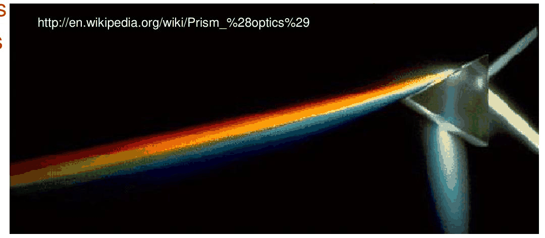
white light as a spectrum of frequencies, separated by a prism

In this notebook

follows the lecture's classical catalogue with small calculations: energy transfer in an elastic collision, a Huygens-principle double slit summed point by point and compared with the Fraunhofer formula, the open-nemo wave equation of a uniform wire (continuous transmission) against the same equation in a closed box (discrete \(k_j = j\pi/L\)), energy exchange between two coupled resonators as a function of detuning, and the dispersion of a glass prism.

Run the notebookEvery number and figure on this page comes from it. Change it, rerun it, take it further.

Download .ipynb View on GitHub

Run it on your own machine

The notebook needs open-nemo (Python ≥ 3.10 and a C++20 compiler; BLAS/LAPACK).

git clone https://github.com/denphi/open-nemo.git && cd open-nemo
python3 -m venv .venv && source .venv/bin/activate
pip install -e ".[notebooks]"
jupyter lab From_Atoms_to_Devices/02_materials_and_quantum_mechanics/04_1_classic_systems.ipynb

Code7 lines · cell 1

import numpy as np
import matplotlib.pyplot as plt
import opennemo as nemo
from opennemo.visualization import style

style.use(notebook=True)
from opennemo.core.units import HBAR2_2M0

1. Why quantum mechanics?#

Section 4 of the course opens with the current again, \(I = q\,n\,v\,A\), and with the observation from Lecture 2.1: the density \(n\) of electrons available for conduction is not the number of atoms per volume (from the crystal structure) times the number of electrons per atom,

n \neq N \times \rho .

"All electrons may be created equally, but they do not behave identically": some are bound to their atoms, some move freely. To understand which, Klimeck first collects what classical physics knows about particles and waves, so that the experiments of Lecture 4.2 can show where it fails.

2. Classical particles#

A classical particle (a billiard ball) has a finite extent and a finite weight, both continuous if the atomic granularity is ignored, and particles are countable with integers. They move according to Newton's laws, and in collisions they exchange energy and momentum continuously, subject only to the conservation of both. For a head-on elastic collision of a ball of mass \(m_1\) and speed \(v_1\) with a ball of mass \(m_2\) at rest, momentum and energy conservation give

v_1' = \frac{m_1 - m_2}{m_1 + m_2}\,v_1, \qquad v_2' = \frac{2m_1}{m_1 + m_2}\,v_1, \qquad \frac{E_2'}{E_1} = \frac{4\,m_1 m_2}{(m_1 + m_2)^2}.

The fraction of energy handed over varies continuously with the mass ratio and reaches 1 only for equal masses. The cell checks the formula by solving the two conservation laws directly.

Code22 lines · cell 3

def collide(m1, m2, v1):
    """Head-on elastic collision with ball 2 at rest: solve momentum and energy conservation."""
    # momentum: m1 v1 = m1 a + m2 b; energy: m1 v1^2 = m1 a^2 + m2 b^2 -> quadratic in b, nontrivial root
    b = 2 * m1 * v1 / (m1 + m2)
    a = v1 - m2 * b / m1
    assert np.isclose(m1 * v1**2, m1 * a**2 + m2 * b**2)
    return a, b


ratio = np.logspace(-2, 2, 201)  # m2 / m1
transfer = np.array([0.5 * r * collide(1.0, r, 1.0)[1] ** 2 / 0.5 for r in ratio])
print(f"largest difference to 4 m1 m2/(m1+m2)^2: {np.max(abs(transfer - 4 * ratio / (1 + ratio) ** 2)):.1e}")
for r in (0.1, 1.0, 10.0):
    print(f"m2/m1 = {r:5.1f}: fraction of the energy transferred {4 * r / (1 + r) ** 2:.3f}")
fig, ax = plt.subplots(figsize=(6, 3.5))
ax.semilogx(ratio, transfer, color=style.OPEN_NEMO)
ax.set(
    xlabel="mass ratio m₂/m₁",
    ylabel="energy fraction E₂′/E₁",
    title="elastic collision: continuous energy transfer",
)
fig.tight_layout();

largest difference to 4 m1 m2/(m1+m2)^2: 2.2e-16
m2/m1 =   0.1: fraction of the energy transferred 0.331
m2/m1 =   1.0: fraction of the energy transferred 1.000
m2/m1 =  10.0: fraction of the energy transferred 0.331

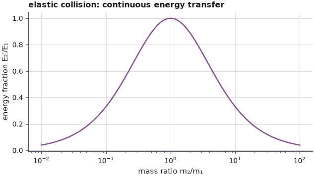
Figure computed by the notebook with open-nemo

A light ball (\(m_2/m_1 = 0.1\)) and a heavy ball (\(m_2/m_1 = 10\)) both take 0.331 of the energy; equal balls take all of it. Keep the shape of \(4m_1m_2/(m_1+m_2)^2\) in mind: the transmission of a quantum wave over a potential step in Lecture 5 has exactly the same form, with wave numbers in place of masses.

3. Propagating waves#

A propagating plane wave obeys the wave equation

\frac{\partial^2 u}{\partial t^2} - c^2 \frac{\partial^2 u}{\partial x^2} = 0,

with the solution \(u = u_0 \sin(kx - \omega t)\) and the phase velocity \(c = \omega/k = \lambda f\). A plane wave has infinite extent and a definite wavelength and frequency, and both can take any value: they are continuous and the waves are not countable. Waves interact by coherent superposition: two waves add up, constructively or destructively, so that one wave can cancel another. Klimeck's examples are noise-cancelling headsets and the muffler of a car, which sends part of the sound along a path half a wavelength longer so that it interferes destructively with itself.

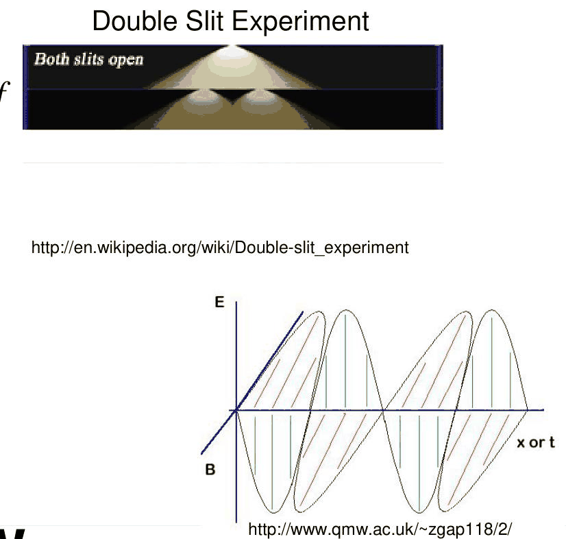
Huygens' principle states that every point of a wavefront acts as a source of a circular wave, and the superposition of these circular waves builds the next wavefront. It explains diffraction: waves go around corners. The double-slit experiment, in which light behind two slits forms bright and dark fringes, is the accepted proof that light is an electromagnetic wave.

Slide 9: double-slit pattern and electromagnetic wave — Slide 9: the double-slit experiment (top) and an electromagnetic wave with its electric and magnetic fields (bottom).

The cell applies Huygens' principle literally. Two slits of width \(a = 10\) µm, \(d = 50\) µm apart, are lit by red light, \(\lambda = 633\) nm. Each slit is replaced by 200 point sources, and the circular waves \(e^{ikr}/\sqrt{r}\) of all 400 sources are summed on a screen \(D = 1\) m away. Far from the slits the sum must reproduce the Fraunhofer formula

I(\theta) \propto \cos^2\!\left(\frac{\pi d \sin\theta}{\lambda}\right) \left[\frac{\sin(\pi a \sin\theta/\lambda)}{\pi a \sin\theta/\lambda}\right]^2,

with fringes \(\lambda D/d\) apart under an envelope whose first zero is at \(\lambda D/a\).

Code30 lines · cell 5

lam, a_slit, d_slit, D = 633e-9, 10e-6, 50e-6, 1.0  # m
k = 2 * np.pi / lam
src = np.concatenate([c + np.linspace(-a_slit / 2, a_slit / 2, 200) for c in (-d_slit / 2, d_slit / 2)])
y = np.linspace(-0.08, 0.08, 4001)  # screen coordinate (m)
r = np.sqrt(D**2 + (y[:, None] - src[None, :]) ** 2)
field = np.sum(np.exp(1j * k * r) / np.sqrt(r), axis=1)
I_huygens = abs(field) ** 2 / np.max(abs(field) ** 2)
s = np.sin(np.arctan(y / D))
I_fraunhofer = np.cos(np.pi * d_slit * s / lam) ** 2 * np.sinc(a_slit * s / lam) ** 2

centre, Ic = y[abs(y) < 0.03], I_huygens[abs(y) < 0.03]
dark = centre[1:-1][(Ic[1:-1] < Ic[:-2]) & (Ic[1:-1] < Ic[2:])]  # dark fringes: zeros of the cos² factor
print(
    f"dark-fringe spacing: Huygens sum {1e3 * np.mean(np.diff(dark)):.2f} mm, λD/d = "
    f"{1e3 * lam * D / d_slit:.2f} mm"
)
print(
    f"envelope zero λD/a = {1e3 * lam * D / a_slit:.1f} mm; "
    f"largest difference Huygens − Fraunhofer {np.max(abs(I_huygens - I_fraunhofer)):.4f}"
)

fig, ax = plt.subplots(figsize=(8, 3.6))
ax.plot(1e3 * y, I_huygens, color=style.OPEN_NEMO, label="Huygens sum of 400 point sources")
ax.plot(1e3 * y, I_fraunhofer, "--", color=style.REFERENCE, lw=1, label="Fraunhofer formula")
ax.plot(1e3 * y, np.sinc(a_slit * s / lam) ** 2, ":", color=style.CONTEXT, label="single-slit envelope")
ax.set(
    xlabel="position on the screen y (mm)", ylabel="intensity (normalized)", title="double slit, λ = 633 nm"
)
ax.legend(frameon=False, fontsize=8, loc="upper right")
fig.tight_layout();

dark-fringe spacing: Huygens sum 12.67 mm, λD/d = 12.66 mm
envelope zero λD/a = 63.3 mm; largest difference Huygens − Fraunhofer 0.0043

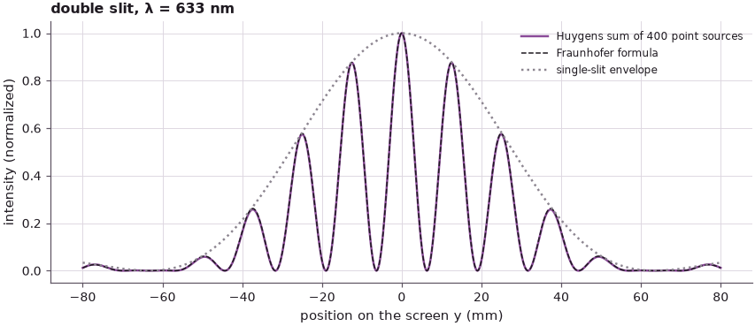
The summed circular waves produce dark fringes 12.67 mm apart, the value \(\lambda D/d = 12.66\) mm predicts, under the single-slit envelope with its first zero at 63.3 mm; the Huygens sum and the formula differ by less than 0.01 of the peak. Note what the pattern requires: every source contributes with its phase \(kr\), and the dark fringes are places where waves from the two slits cancel. Particles that go through one slit or the other could not produce them.

4. Standing waves#

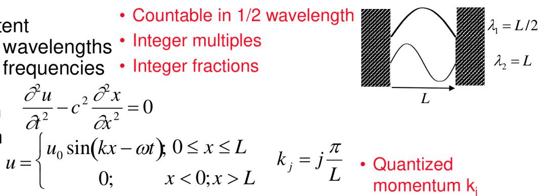
When a wave is confined to \(0 \le x \le L\), for example a guitar string clamped at both ends, it must vanish at the ends. Only waves that fit an integer number of half wavelengths into \(L\) survive:

u_j(x, t) = u_0 \sin(k_j x)\cos(\omega_j t), \qquad k_j = j\,\frac{\pi}{L}, \qquad \lambda_j = \frac{2L}{j}, \qquad j = 1, 2, 3, \ldots

A standing wave has a finite extent, discrete wavelengths and discrete frequencies, and it is countable in half wavelengths. The momentum, proportional to \(k_j\), is quantized. (The slide labels the two waves it draws \(\lambda_1 = L/2\) and \(\lambda_2 = L\); it is half the fundamental wavelength that fits into the box, \(\lambda_1/2 = L\).)

Slide 10: standing waves between two walls — Slide 10: standing waves in a box of length L: the wave equation, its confined solution and the quantized wave numbers k_j = jπ/L.

open-nemo's effective-mass model solves the same equation. Its Hamiltonian is the discretized operator \(-(\hbar^2/2m)\,d^2/dx^2\), so its eigenvalues are \(E = (\hbar^2/2m)k^2\) and its eigenvectors are the allowed wave shapes; the wave equation of a string has the same spatial operator, with \(\omega = c k\) in place of \(E \propto k^2\). The cell compares two cases with \(m = m_0\). A uniform wire that continues into semi-infinite leads at both ends supports propagating waves at every energy: open-nemo's transmission is 1 throughout. The same wire cut to a box of \(L = 10\) nm supports only discrete waves. On a grid of spacing \(\Delta x\) the walls sit one grid point outside the last site, so the box is \(L + \Delta x\) long.

Code38 lines · cell 7

mat = nemo.structures.materials.EffectiveMassMaterial("free", 1.0, 1.0, conduction_band_edge=0.0)
dx = 0.01
wire = nemo.Heterostructure1D([nemo.Layer(mat, 5.0), nemo.Layer(mat, 10.0), nemo.Layer(mat, 5.0)], spacing=dx)
E = np.linspace(0.001, 1.0, 400)
T = nemo.Transport(wire.hamiltonian).transmission(E)
print(f"uniform wire: transmission between {T.min():.6f} and {T.max():.6f} for 0.001 eV < E < 1 eV")

box = nemo.Heterostructure1D([nemo.Layer(mat, 10.0)], spacing=dx)
st = nemo.eigenstates(box.hamiltonian.sparse, num=6)
order = np.argsort(st["energies"])
Ej, vecs = np.asarray(st["energies"])[order], np.asarray(st["vectors"])[:, order]
kj = np.sqrt(Ej / HBAR2_2M0)
L_eff = box.num_sites * dx + dx
print(f"box: {box.num_sites} sites, effective length {L_eff:.2f} nm")
print(" j    k_j (nm⁻¹)   jπ/L (nm⁻¹)   k_j L/π")
for j, kv in enumerate(kj, start=1):
    print(f"{j:2d}   {kv:10.5f}   {j * np.pi / L_eff:11.5f}   {kv * L_eff / np.pi:8.5f}")
k6 = 6 * np.pi / L_eff
print(
    f"relative error of k_6: {100 * (1 - kj[5] / k6):.4f} %; (k Δx)²/24 = {100 * (k6 * dx) ** 2 / 24:.4f} %"
)

fig, (a1, a2) = plt.subplots(1, 2, figsize=(11, 3.8))
a1.plot(E, T, color=style.OPEN_NEMO)
a1.set(
    xlabel="energy E (eV)", ylabel="transmission T", ylim=(0, 1.1), title="open wire: every wave propagates"
)
x_full = np.linspace(0, L_eff, 400)
for j, c in zip(range(4), style.sweep(4)):
    v = vecs[:, j].real / np.max(abs(vecs[:, j]))
    v *= np.sign(v[np.argmax(abs(v[: len(v) // (j + 1)]))])
    a2.plot(box.x + dx, 2.5 * j + v, color=c, label=f"j = {j + 1}")
    a2.plot(x_full, 2.5 * j + np.sin((j + 1) * np.pi * x_full / L_eff), ":", color=style.REFERENCE, lw=1)
a2.set(
    xlabel="position x (nm)", ylabel="mode shape (offset)", title="closed box: k_j = jπ/L (dotted: sin k_j x)"
)
a2.legend(frameon=False, fontsize=8, loc="upper right")
fig.tight_layout();

uniform wire: transmission between 1.000000 and 1.000000 for 0.001 eV < E < 1 eV
box: 1000 sites, effective length 10.01 nm
 j    k_j (nm⁻¹)   jπ/L (nm⁻¹)   k_j L/π
 1      0.31385       0.31385    1.00000
 2      0.62769       0.62769    2.00000
 3      0.94153       0.94154    2.99999
 4      1.25537       1.25538    3.99997
 5      1.56921       1.56923    4.99995
 6      1.88304       1.88307    5.99991
relative error of k_6: 0.0015 %; (k Δx)²/24 = 0.0015 %

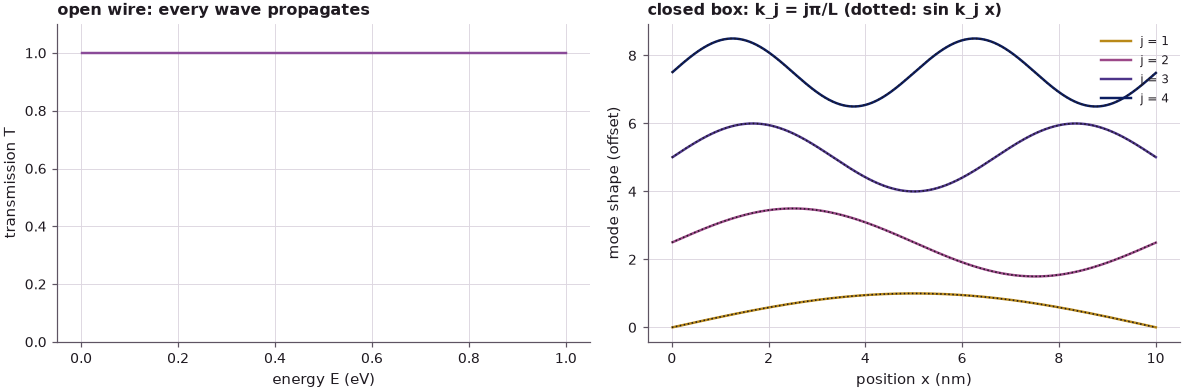
The open wire transmits every wave between 0.001 and 1 eV with \(T = 1\) to six digits: a continuum of propagating waves. The box of 1000 sites (\(L + \Delta x = 10.01\) nm) keeps only the waves with \(k_j L/\pi = 1, 2, 3, \ldots\); the discretization lowers the sixth one by only 0.0015 %, the error of the finite-difference second derivative: the discrete energy is \(E = (\hbar^2/m\Delta x^2)(1 - \cos k\Delta x)\), which makes \(k\) too small by \((k\Delta x)^2/24\). The mode shapes are the sine functions of the formula. Nothing in the calculation knows whether the wave is a string, a sound wave or an electron: confinement alone makes the wave numbers discrete.

Coupled resonators must be in tune#

A standing wave is a resonator, and one resonator can drive another: a guitar string drives the wooden body, which radiates the sound. Energy passes from one to the other, but only efficiently if the two are in tune. Klimeck connects this with energy and momentum conservation, which will reappear as selection rules for electrons and photons. The cell models two oscillators of frequencies \(\omega_1\) and \(\omega_2\) joined by a weak spring of strength \(\kappa\),

\ddot x_1 = -\omega_1^2 x_1 - \kappa(x_1 - x_2), \qquad \ddot x_2 = -\omega_2^2 x_2 - \kappa(x_2 - x_1),

starts the first one and records the largest share \(E_2/(E_1 + E_2)\) of the oscillator energies that ever reaches the second. Coupled-mode theory predicts \(g^2/[g^2 + (\Delta/2)^2]\), with the detuning \(\Delta = \omega_2 - \omega_1\) and the coupling rate \(g = \kappa/2\omega\).

Code35 lines · cell 9

w1, kappa = 2 * np.pi * 1.0, 0.02 * (2 * np.pi) ** 2  # rad/s; coupling spring (1/s^2)
t = np.linspace(0, 400, 40001)


def max_transfer(w2):
    """Exact normal-mode solution, resonator 1 displaced and released; max energy fraction in resonator 2."""
    K = np.array([[w1**2 + kappa, -kappa], [-kappa, w2**2 + kappa]])
    lam_, modes = np.linalg.eigh(K)
    amp = modes.T @ np.array([1.0, 0.0])  # initial displacement in normal-mode coordinates
    x2 = (modes[1] * amp) @ np.cos(np.sqrt(lam_)[:, None] * t)
    v2 = -(modes[1] * amp * np.sqrt(lam_)) @ np.sin(np.sqrt(lam_)[:, None] * t)
    x1 = (modes[0] * amp) @ np.cos(np.sqrt(lam_)[:, None] * t)
    v1 = -(modes[0] * amp * np.sqrt(lam_)) @ np.sin(np.sqrt(lam_)[:, None] * t)
    e1, e2 = 0.5 * v1**2 + 0.5 * w1**2 * x1**2, 0.5 * v2**2 + 0.5 * w2**2 * x2**2
    return np.max(e2 / (e1 + e2))


detune = np.linspace(-0.06, 0.06, 61) * w1
frac = np.array([max_transfer(w1 + dw) for dw in detune])
g = kappa / (2 * w1)
for dw in (0.0, 0.01, 0.03):
    print(
        f"detuning Δ/ω₁ = {dw:4.2f}: max transfer {max_transfer(w1 * (1 + dw)):.3f}, "
        f"coupled-mode estimate {g**2 / (g**2 + (dw * w1 / 2) ** 2):.3f}"
    )
fig, ax = plt.subplots(figsize=(6.5, 3.6))
ax.plot(detune / w1, frac, color=style.OPEN_NEMO, label="exact normal modes")
ax.plot(
    detune / w1, g**2 / (g**2 + (detune / 2) ** 2), "--", color=style.REFERENCE, label="coupled-mode estimate"
)
ax.set(
    xlabel="detuning Δ/ω₁", ylabel="max energy fraction in resonator 2", title="resonators must be in tune"
)
ax.legend(frameon=False, fontsize=8)
fig.tight_layout();

detuning Δ/ω₁ = 0.00: max transfer 1.000, coupled-mode estimate 1.000
detuning Δ/ω₁ = 0.01: max transfer 0.806, coupled-mode estimate 0.800
detuning Δ/ω₁ = 0.03: max transfer 0.314, coupled-mode estimate 0.308

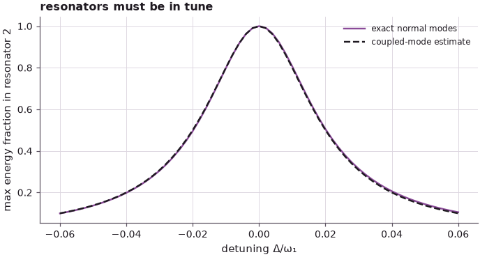
Tuned resonators exchange all of the energy (1.000 in the exact solution). A detuning of 1 % already limits the transfer to 0.806 (coupled-mode estimate 0.800), and at 3 % only 0.314 arrives (estimate 0.308). The width of the resonance is set by the coupling, \(\Delta \approx 2g\).

5. White light and its spectrum#

The last classical observation is chromatography: white light consists of a broad spectrum of colours, each colour is a wave of a particular frequency, and a prism separates them because the refractive index of glass depends on the wavelength.

Slide 12: a prism separating white light into colours — Slide 12: a prism dissects white light into its frequency components.

For a 60° prism of BK7 glass at minimum deviation the deflection angle is \(\delta = 2\arcsin[n(\lambda)\sin(A/2)] - A\), with the Sellmeier formula \(n^2 = 1 + \sum_i B_i\lambda^2/(\lambda^2 - C_i)\) (Schott catalogue coefficients).

Code17 lines · cell 11

B_ = (1.03961212, 0.231792344, 1.01046945)
C_ = (0.00600069867, 0.0200179144, 103.560653)  # µm²
lam_um = np.linspace(0.40, 0.70, 61)
n = np.sqrt(1 + sum(b * lam_um**2 / (lam_um**2 - c) for b, c in zip(B_, C_)))
A = np.radians(60.0)
delta = np.degrees(2 * np.arcsin(n * np.sin(A / 2)) - A)
f_THz = 299792458 / (lam_um * 1e-6) / 1e12
for l_, n_, d_, f_ in zip(lam_um[::20], n[::20], delta[::20], f_THz[::20]):
    print(f"λ = {1e3 * l_:.0f} nm (f = {f_:.0f} THz): n = {n_:.4f}, deviation {d_:.2f}°")
fig, ax = plt.subplots(figsize=(6.5, 3.6))
ax.scatter(1e3 * lam_um, delta, c=lam_um, cmap="turbo", s=18)
ax.set(
    xlabel="wavelength λ (nm)",
    ylabel="deviation δ (degrees)",
    title="60° BK7 prism: each colour leaves at its own angle",
)
fig.tight_layout();

λ = 400 nm (f = 749 THz): n = 1.5308, deviation 39.89°
λ = 500 nm (f = 600 THz): n = 1.5214, deviation 39.05°
λ = 600 nm (f = 500 THz): n = 1.5163, deviation 38.60°
λ = 700 nm (f = 428 THz): n = 1.5131, deviation 38.32°

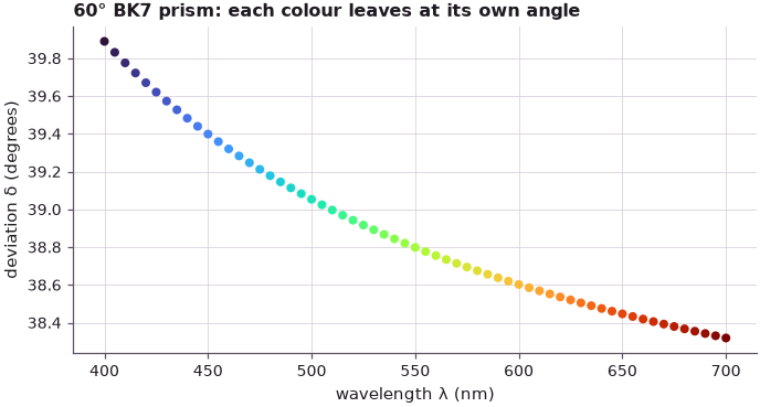
Violet light (400 nm, 749 THz) is bent by 39.89°, red light (700 nm, 428 THz) by 38.32°, so the colours fan out by 1.6°. A spectrum can therefore be measured, and Klimeck's closing question is whether such spectra contain information. Lecture 4.2 answers it: the spectra of hot bodies and of atoms are where classical physics fails.

Summary#

The density of conducting electrons is not \(N\times\rho\); to find it, the behaviour of electrons as particles and as waves has to be understood.
Classical particles are countable and exchange energy continuously; an elastic collision transfers the fraction \(4m_1m_2/(m_1+m_2)^2\) (0.331 for a mass ratio of 10).
Propagating waves have continuous wavelengths and interfere. A Huygens sum of 400 point sources reproduces the double-slit fringes, 12.67 mm apart for 633 nm light, 50 µm slit spacing and 1 m distance. open-nemo transmits every wave through a uniform open wire (\(T = 1\)).
Standing waves are discrete: in open-nemo's 10 nm box the wave numbers are \(k_j = j\pi/L\) to 0.0015 % up to \(j = 6\). Coupled resonators exchange all of their energy when in tune and only 0.314 of it when detuned by 3 %.
A prism separates white light by frequency (deviation from 38.3° to 39.9° for BK7 across the visible).

Exercises#

Make the slits of section 3 wider (\(a = 25\) µm). How many bright fringes fit under the central envelope now? Derive the number \(2d/a - 1\).
Repeat the box calculation of section 4 with \(\Delta x = 0.05\) nm and \(\Delta x = 0.1\) nm and compare the relative error of \(k_6\) with \((k\Delta x)^2/24\).
A guitar string of length 0.648 m is tuned to 82.4 Hz. What is the wave speed on it, and what are the frequencies of its first four standing waves? Which of them is "in tune" with a body resonance at 247 Hz?