Lecture 1.5

nanoHUB access and tool demo

In the lecture

nanoHUB, the science gateway where the course's simulation tools run in a web browser
its reach: more than 23,000 simulation users a year, over 2 million visitors, more than 945 simulation apps and 8,700 resources, used in over 3,840 classes at 185 institutions
a live demonstration of the tools
the learning outcomes of the course again: explain, relate, speak the language of device engineers, be ready for device research — and operate advanced simulation tools

In this notebook

we do the tool demonstration with open-nemo's three small apps, the ones behind its interactive explorer: the bulk band structure of a crystal, the ballistic transmission of a silicon nanowire, and the current–voltage curve of a resonant tunneling diode. Each result is checked against a number it must reproduce — a band gap, the number of open channels, a resonance energy — and each is then varied once, the way the nanoHUB tools are meant to be used.

Run the notebookEvery number and figure on this page comes from it. Change it, rerun it, take it further.

Download .ipynb View on GitHub

Run it on your own machine

The notebook needs open-nemo (Python ≥ 3.10 and a C++20 compiler; BLAS/LAPACK).

git clone https://github.com/denphi/open-nemo.git && cd open-nemo
python3 -m venv .venv && source .venv/bin/activate
pip install -e ".[notebooks]"
jupyter lab From_Atoms_to_Devices/01_introduction/01_5_nanohub_access_and_tool_demo.ipynb

Code10 lines · cell 1

import numpy as np
import matplotlib.pyplot as plt
import opennemo as nemo
from opennemo.visualization import style

style.use(notebook=True)
from opennemo.devices import app

props = nemo.structures.properties
G0 = nemo.core.units.G0           # conductance quantum 2q²/h (S)

1. nanoHUB#

nanoHUB.org started at Purdue as a place to run research codes for nanotechnology from a browser, without installing anything, and grew into a gateway for simulation, teaching material and courses. The numbers on slide 2 measure its reach: more than 23,000 users run simulations each year, out of more than 2 million visitors; more than 945 simulation apps and 8,700 resources, more than 170 courses; over 100,000 students in more than 3,840 classes at 185 institutions; more than 3,400 papers cite it (h-index 135), and the service runs with 99.4 % uptime. The course's own tools — band structure labs, the PN junction lab of Lecture 1.4, RTD and nanowire simulators built on NEMO — are among them.

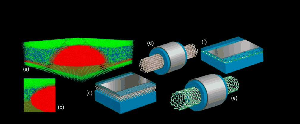
Slide 2: nanoHUB in numbers — Slide 2: nanoHUB's usage — simulation users, visitors, apps, resources, courses, classes, citations and uptime.

The demonstration itself is live in the video. Here open-nemo plays the part of the tools; the same three calculations are available as interactive apps (app.launch() in a notebook).

2. Tool 1: the band structure of a crystal#

app.band_structure diagonalizes the sp3d5s* tight-binding Hamiltonian of a bulk crystal along a path through the Brillouin zone and reports the gap, whether it is direct, and where the conduction-band minimum is. Silicon's gap must be indirect, with the minimum about 85 % of the way from Γ to X; its size must match the measured 1.12 eV at room temperature.

Code15 lines · cell 3

runs = {"Si": app.band_structure(),
        "Ge": app.band_structure(material="Ge"),
        "GaAs": app.band_structure(parameter_set="nemo5_sp3d5s_so", material="GaAs")}
fig, axes = plt.subplots(1, 3, figsize=(12, 4), sharey=True)
print("material  parameter set        gap TB (eV)  registry (eV)  direct  k_cbm (2π/a)")
for ax, (name, r) in zip(axes, runs.items()):
    ax.plot(r["distance"], r["bands"], color=style.OPEN_NEMO, lw=0.9)
    for x, _ in r["ticks"]:
        ax.axvline(x, color=style.CONTEXT, lw=0.5)
    ax.set_xticks([x for x, _ in r["ticks"]], [lab.replace("G", "Γ") for _, lab in r["ticks"]])
    ax.set(xlim=(r["distance"][0], r["distance"][-1]), ylim=(-4, 5), title=f"{name} ({r['parameter_set']})")
    print(f"{name:8s}  {r['parameter_set']:18s}  {r['gap']:11.3f}  {props.value(name, 'band_gap'):13.3f}  "
          f"{str(r['direct']):6s}  {np.round(r['k_cbm'], 3)}")
axes[0].set_ylabel("energy (eV)")
fig.tight_layout()

material  parameter set        gap TB (eV)  registry (eV)  direct  k_cbm (2π/a)
Si        boykin2004_sp3d5s         1.147          1.125  False   [0.813 0.    0.   ]
Ge        boykin2004_sp3d5s         0.754          0.663  False   [0.5 0.5 0.5]
GaAs      nemo5_sp3d5s_so           1.531          1.422  True    [0. 0. 0.]

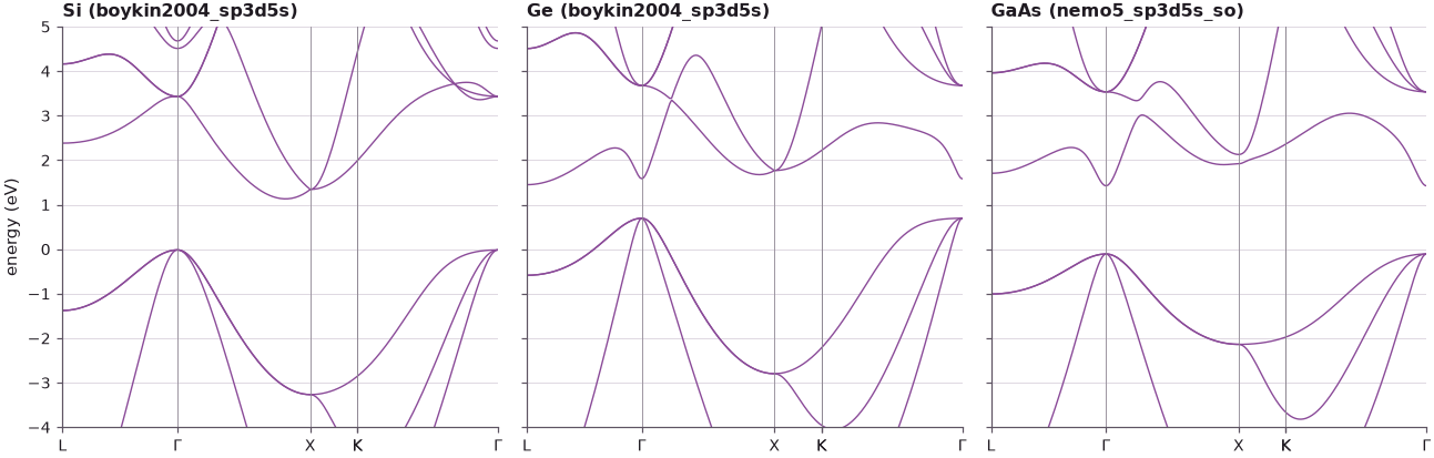
Figure computed by the notebook with open-nemo

Silicon comes out indirect with the minimum at 0.81 of Γ–X, germanium indirect (minimum at L), GaAs direct. The silicon gap is within 0.03 eV of the registry's room-temperature value; the germanium gap is 0.09 eV larger (close to its low-temperature value, 0.74 eV), and the GaAs gap 0.11 eV larger because this run leaves out spin and with it the spin–orbit splitting (see Lecture 1.3). Checking such numbers before trusting a tool is part of operating it. This is what "atomistic" buys: the whole Brillouin zone, not just one valley.

3. Tool 2: a silicon nanowire, one channel at a time#

app.nanowire_transmission builds a hydrogen-passivated [100] silicon wire, two conventional cells (1.09 nm) square, in the sp3s* model, and computes its ballistic transmission. In a perfect wire every electron that enters a propagating mode leaves through it, so $T(E)$ must equal the number of open channels of the lead, and the Landauer conductance is $G = G_0\,T$ with $G_0 = 2q^2/h = 77.5$ µS. Then a 0.3 eV barrier is put in the middle of the wire.

Code21 lines · cell 5

clean = app.nanowire_transmission()
# the barrier needs a longer wire (8 cells) so that its tails stay out of the contact slabs
barrier = app.nanowire_transmission(barrier=0.3, length_cells=8, energies=clean["energies"])
e, t, modes = clean["energies"], clean["transmission"], clean["modes"]
print(f"{clean['orbitals']} orbitals, {clean['length_nm']:.2f} nm long")
print(f"largest |T - number of open channels| without a barrier: {np.max(np.abs(t - modes)):.2e}")
k = np.argmin(np.abs(e - clean["mu"]))
kt = nemo.core.units.KB * 300.0
minus_dfde = 1 / (4 * kt * np.cosh((e - clean["mu"]) / (2 * kt)) ** 2)        # -df/dE (1/eV)
print(f"T(mu = {clean['mu']:.3f} eV) = {t[k]:.2f} channels: G0 x T = {1e6 * G0 * t[k]:.0f} µS at 0 K")
print(f"tool's 300 K conductance {1e6 * clean['conductance']:.0f} µS; G0 ∫T(-df/dE)dE on this grid "
      f"= {1e6 * G0 * np.trapezoid(t * minus_dfde, e):.0f} µS")
print(f"with the 0.3 eV barrier: {1e6 * barrier['conductance']:.0f} µS at its own best energy")

fig, ax = plt.subplots(figsize=(7, 3.8))
ax.plot(e, modes, color=style.CONTEXT, ls="--", lw=1, label="open channels of the lead")
ax.plot(e, t, color=style.OPEN_NEMO, label="T(E), perfect wire")
ax.plot(e, barrier["transmission"], color=style.REFERENCE, lw=1, label="T(E), 0.3 eV barrier")
ax.set(xlabel="energy E (eV)", ylabel="transmission T(E)")
ax.legend(fontsize=8)
fig.tight_layout()

640 orbitals, 2.17 nm long
largest |T - number of open channels| without a barrier: 8.49e-09
T(mu = 1.801 eV) = 9.00 channels: G0 x T = 697 µS at 0 K
tool's 300 K conductance 572 µS; G0 ∫T(-df/dE)dE on this grid = 572 µS
with the 0.3 eV barrier: 110 µS at its own best energy

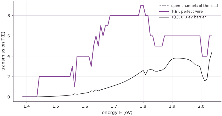
Without a barrier the transmission is the staircase of open channels, to round-off: each subband of the 1 nm wire contributes exactly one $G_0$. At room temperature the conductance is the staircase averaged over a few $k_BT$ around $\mu$, $G = G_0\int T(E)\,(-\partial f/\partial E)\,dE$, which is why the tool reports less than nine $G_0$; the printed integral reproduces its value. The barrier removes the lowest steps and rounds the others: electrons below its top must tunnel. Conductance quantization, subbands set by the cross-section, and tunneling are all in this one plot.

4. Tool 3: a resonant tunneling diode#

app.rtd_iv computes the current density of a GaAs/Al${0.3}$Ga${0.7}$As double-barrier diode (3 nm barriers, a 5 nm well, contacts doped $10^{18}$ cm⁻³): the NEGF transmission at each bias, with the bias dropped linearly over the barriers and the well, and the Tsu–Esaki current. A current peak needs the well's resonance to sit in the energy window of the emitter's electrons; the bias lowers the well by about half the applied voltage, so a first estimate for the peak is $V \approx 2(E_1 - E_F)/q$ and for the end of the current drop $V \approx 2E_1/q$, with $E_1$ the resonance energy at zero bias, measured from the emitter band edge.

Code21 lines · cell 7

gaas = nemo.structures.materials.effective_mass("GaAs")
algaas = nemo.structures.materials.effective_mass("AlGaAs", x=0.3)
dbl = nemo.Heterostructure1D([nemo.Layer(gaas, 20), nemo.Layer(algaas, 3), nemo.Layer(gaas, 5),
                              nemo.Layer(algaas, 3), nemo.Layer(gaas, 20)], spacing=0.1)
res = nemo.resonances(dbl)
e1 = res["energy"][np.argmax(res["energy"] > 0)]
dev = nemo.Heterostructure1D([nemo.Layer(gaas, 20, donors=1e18)], spacing=0.1)
ef = dev.contact_fermi_level("left", 300.0)
print(f"E_1 = {1e3 * e1:.1f} meV (width {1e3 * res['width'][np.argmax(res['energy'] > 0)]:.2f} meV), "
      f"E_F = {1e3 * ef:.1f} meV above the band edge")
print(f"estimates: peak near 2(E_1 - E_F) = {2 * (e1 - ef):.3f} V, "
      f"current drop ends near 2 E_1 = {2 * e1:.3f} V")

curves = {T: app.rtd_iv(temperature=T) for T in (300.0, 77.0)}
fig, ax = plt.subplots(figsize=(7, 3.8))
for c, (T, r) in zip((style.OPEN_NEMO, style.REFERENCE), curves.items()):
    ax.plot(r["bias"], r["current"], "o-", ms=3, color=c, label=f"{T:.0f} K")
    print(f"{T:5.0f} K: peak at {r['peak']:.2f} V, peak-to-valley ratio {r['peak_to_valley']:.1f}")
ax.set(xlabel="bias V (V)", ylabel="current density J (A/cm²)")
ax.legend(fontsize=8)
fig.tight_layout()

E_1 = 74.3 meV (width 3.85 meV), E_F = 41.9 meV above the band edge
estimates: peak near 2(E_1 - E_F) = 0.065 V, current drop ends near 2 E_1 = 0.149 V
  300 K: peak at 0.10 V, peak-to-valley ratio 6.3
   77 K: peak at 0.12 V, peak-to-valley ratio 17.4

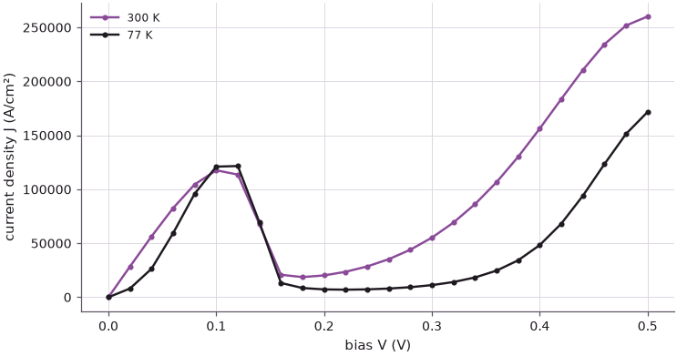
The peak lies between the two estimates, as it should for a resonance that enters the emitter's Fermi sea from above and leaves it at the band edge. Cooling to 77 K sharpens the emitter's Fermi edge and raises the peak-to-valley ratio, because the valley current in this model is carried by electrons in the thermal tail that reach the second resonance or pass over the barriers. Lecture 2 returns to this device: whether the valley current comes from scattering or from the band structure was the question that NEMO answered.

Summary#

nanoHUB delivers simulation tools through a browser to tens of thousands of users a year; the course uses them, and open-nemo provides the same kind of calculations in a notebook.
The band-structure tool reproduces the indirect gaps of Si and Ge and the direct gap of GaAs; the gap values differ from the room-temperature ones by 0.02–0.11 eV, for known reasons.
In a perfect nanowire the transmission equals the number of open channels exactly, and $G = G_0 T$; a barrier turns the staircase into tunneling.
The RTD's current peak lies between the estimates $2(E_1 - E_F)/q$ and $2E_1/q$ from its zero-bias resonance; cooling raises the peak-to-valley ratio.

Exercises#

Run the band-structure tool for Si with vogl1983_sp3s instead of boykin2004_sp3d5s. Where is the conduction-band minimum now, and why does it matter for a transistor?
Make the nanowire three cells wide. How many channels are open 0.2 eV above the lowest subband, and how does the lowest subband move?
Change the RTD barriers from 3 nm to 2 nm and 4 nm. How do the peak current and the peak-to-valley ratio change? Relate the peak current to the width of $E_1$.