Lecture 23.3

Theory of stress and strain — internal forces: stress

In the lecture

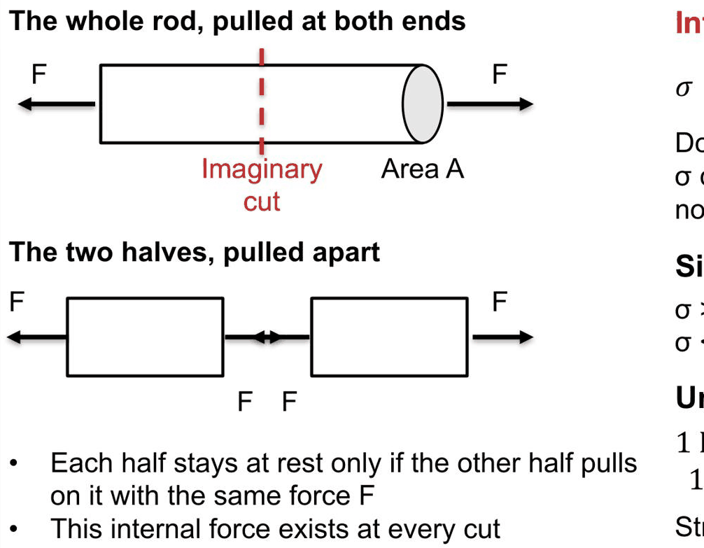
An imaginary cut through a pulled rod: each half stays at rest only because the other half pulls on it, so an internal force acts across every cut.
Stress is that internal force per area, $\sigma = F/A$: it describes the material at a point, not the size of the sample. Positive is tension, negative compression.
Units and sizes: 1 GPa ≈ 10$^4$ atm; strained semiconductor layers carry 0.1–2 GPa, 1,000 to 20,000 atmospheres. Displacements can be seen; forces cannot.
Pressure pushes equally on every face, $\sigma_{xx} = \sigma_{yy} = \sigma_{zz} = -p$; a force along a face is shear stress, which tilts the block.
The stress tensor $\sigma_{ij} = \mathrm{d}F_i/\mathrm{d}A_j$ (force direction $i$, face normal $j$), symmetric because there is no net torque; at a free surface normal to $z$, $\sigma_{xz} = \sigma_{yz} = \sigma_{zz} = 0$.

In this notebook

You pull a GaAs rod with open-nemo's finite-element elasticity solver (opennemo.solvers.elasticity) and check that the stress is the same at every cut and independent of the cross-section; compress a cube hydrostatically and drag the top face of a block to produce pressure and shear stress; compute the force on a face from the stress tensor; and verify the free-surface condition on a strained InAs and In${0.2}$Ga${0.8}$As layer on GaAs, whose stress you convert to atmospheres.

Run the notebookEvery number and figure on this page comes from it. Change it, rerun it, take it further.

Download .ipynb View on GitHub

Run it on your own machine

The notebook needs open-nemo (Python ≥ 3.10 and a C++20 compiler; BLAS/LAPACK).

git clone https://github.com/denphi/open-nemo.git && cd open-nemo
python3 -m venv .venv && source .venv/bin/activate
pip install -e ".[notebooks]"
jupyter lab From_Atoms_to_Devices/09_stress_and_strain/23_3_internal_forces_stress.ipynb

Code9 lines · cell 1

import numpy as np
import matplotlib.pyplot as plt
import opennemo as nemo
from opennemo.visualization import style
from opennemo.models import kp
from opennemo.solvers import elasticity as E
from opennemo.solvers.poisson import Grid

style.use(notebook=True)

1. Forces inside a solid: the imaginary cut#

Lecture 23.2 described how far atoms move. This lecture asks what forces the atoms feel once they have been moved. Pull a rod at both ends with a force $F$ and imagine a cut through it. The cut does not exist; it is a bookkeeping device. Each half of the rod stays at rest only if the other half pulls on it with the same force $F$, so that internal force is transmitted by all the atoms that straddle the cut, and it exists at every cut, wherever it is placed. The internal force per area is the stress,

\sigma = \frac{F}{A} .

A rod of twice the cross-section needs twice the force for the same stretch, but the stress is the same: $\sigma$ describes the material at a point, not the size of the sample. $\sigma > 0$ is tension (the halves pull on each other), $\sigma < 0$ compression (they push). The unit is the pascal, $1\ \mathrm{Pa} = 1\ \mathrm{N/m^2}$, and $1\ \mathrm{GPa} = 10^9\ \mathrm{Pa} \approx 10^4$ atmospheres. Strained semiconductor layers carry 0.1 to 2 GPa, 1,000 to 20,000 times the air pressure we breathe.

Slide 3: a pulled rod and an imaginary cut — Slide 3. Top: the whole rod, pulled at both ends. Bottom: the two halves after an imaginary cut; each must pull on the other with the force $F$ for both to stay at rest.

Klimeck stresses an asymmetry between the two concepts: strain is displacement, and displacement can be seen (in a microscope, in X-ray diffraction); force cannot be seen. A simulation therefore obtains the stress from the computed displacements, through the material law of Lecture 23.4. The cell below does this with the finite-element solver elasticity.Elasticity: a GaAs rod, 10 nm long, is stretched by 0.1 % (its right end is moved by 0.01 nm along $x$ while the left end is held), its sides are free, and the stress tensor is evaluated in every finite element. The internal force across a cut at position $x$ is $F(x) = \int \sigma_{xx}\,\mathrm{d}A$ over that cross-section. With stress in GPa and area in nm² the force comes out in nN ($1\ \mathrm{GPa \cdot nm^2} = 1\ \mathrm{nN}$).

Code20 lines · cell 3

gaas = kp.material("GaAs")                                       # Vurgaftman 2001 parameters
C_gaas = E.cubic_stiffness(gaas.c11, gaas.c12, gaas.c44)         # 6x6 stiffness (GPa), Lecture 23.4

def pull_rod(length=10.0, width=2.0, height=2.0, stretch=0.01, h=0.5):
    # rod along x; left face held in x, right face moved by `stretch` nm; sides free
    g = Grid(*(np.linspace(0, s, int(round(s / h)) + 1) for s in (length, width, height)))
    el = E.Elasticity(g, C_gaas)
    X = g.nodes
    el.fix(np.isclose(X[:, 0], 0), (0,), 0.0)
    el.fix(np.isclose(X[:, 0], length), (0,), stretch)
    el.fix(np.flatnonzero(np.all(np.isclose(X, [0, 0, 0]), axis=1)), (1, 2), 0.0)   # no rigid motion
    el.fix(np.flatnonzero(np.all(np.isclose(X, [0, width, 0]), axis=1)), (2,), 0.0)
    return el, el.solve()

el, r = pull_rod()
xc = el.cell_centers[:, 0]
cuts = np.unique(np.round(xc, 6))
F_cut = np.array([r.stress[np.isclose(xc, c), 0, 0].mean() * 2.0 * 2.0 for c in cuts])   # nN
print(f"σ_xx in the rod: {r.stress[:, 0, 0].min():.4f} to {r.stress[:, 0, 0].max():.4f} GPa")
print(f"force across the {len(cuts)} cuts: {F_cut.min():.3f} to {F_cut.max():.3f} nN")

σ_xx in the rod: 0.0862 to 0.0862 GPa
force across the 20 cuts: 0.345 to 0.345 nN

Code8 lines · cell 4

print(" cross-section   force (nN)   stress σ_xx (GPa)   strain ε_xx (%)")
for w, hgt in ((2.0, 2.0), (4.0, 2.0), (4.0, 4.0)):
    el_w, r_w = pull_rod(width=w, height=hgt)
    sig, eps = r_w.stress[:, 0, 0].mean(), r_w.strain[:, 0, 0].mean()
    print(f"  {w:.0f} nm × {hgt:.0f} nm   {sig * w * hgt:9.3f}   {sig:15.4f}   {100 * eps:14.3f}")
GPa_in_atm = 1e9 / 101325.0
print(f"1 GPa = {GPa_in_atm:.0f} atm;  0.1 GPa = {0.1 * GPa_in_atm:,.0f} atm,  "
      f"2 GPa = {2 * GPa_in_atm:,.0f} atm")

 cross-section   force (nN)   stress σ_xx (GPa)   strain ε_xx (%)
  2 nm × 2 nm       0.345            0.0862            0.100
  4 nm × 2 nm       0.690            0.0862            0.100
  4 nm × 4 nm       1.380            0.0862            0.100
1 GPa = 9869 atm;  0.1 GPa = 987 atm,  2 GPa = 19,738 atm

The stress, 0.0862 GPa at a strain of 0.1 %, is the same in every element, and the force across all 20 cuts is the same, 0.345 nN: this is the statement that each half pulls on the other with the same force wherever the cut is made. Doubling the cross-section doubles the force (0.690 nN), and quadrupling it quadruples it (1.380 nN), while the stress stays 0.0862 GPa. The conversion factor is 1 GPa = 9,869 atm, so the slide's range of 0.1–2 GPa is 987 to 19,738 atm.

2. Pressure from all sides, and shear along a face#

Two loads are special. Hydrostatic pressure $p$ pushes inward equally on every face, so the force on each face is normal to it, and

\sigma_{xx} = \sigma_{yy} = \sigma_{zz} = -p ,

with the minus sign because pressure compresses. A force $F_\parallel$ along a face of area $A$, as when the top of a block is dragged sideways, is a shear stress $\tau = F_\parallel/A$. The block tilts: its angles change, which is the shear strain of Lecture 23.2. In general every face carries a normal and a shear part at the same time, and one bookkeeping object is needed for all of them: the stress tensor.

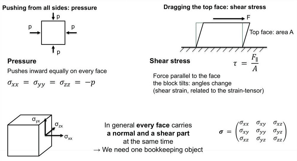
Slide 4: pressure from all sides and shear along a face — Slide 4. Left: dragging the top face, a force parallel to the face, tilts the block (shear stress $\tau$). Right: pressure pushes inward on every face, $\sigma_{xx} = \sigma_{yy} = \sigma_{zz} = -p$.

Both loads are easy to impose on a finite-element block of GaAs. For pressure, every surface node of a 2 nm cube is moved towards the centre as a uniform compression by 0.5 %. For shear, a 2 nm high slab, periodic in $x$ and $y$, is held at the bottom while its top face is moved by 0.02 nm along $x$.

Code11 lines · cell 6

g = Grid(*(np.linspace(0, 2, 5),) * 3)
el = E.Elasticity(g, C_gaas)
X = g.nodes
surface = np.any(np.isclose(X, 0) | np.isclose(X, 2), axis=1)
for node in np.flatnonzero(surface):                             # u = -0.005 (x - centre) on the surface
    el.fix([node], (0, 1, 2), -0.005 * (X[node] - 1.0))
r_p = el.solve()
sig_p = r_p.stress.mean(axis=0)
print("hydrostatic compression by 0.5 %: stress tensor (GPa)\n", np.round(sig_p, 4))
print(f"pressure p = {-np.trace(sig_p) / 3:.4f} GPa = {-np.trace(sig_p) / 3 * GPa_in_atm:,.0f} atm, "
      f"volume change Tr ε = {100 * np.trace(r_p.strain.mean(axis=0)):.2f} %")

hydrostatic compression by 0.5 %: stress tensor (GPa)
 [[-1.1765 -0.      0.    ]
 [-0.     -1.1765  0.    ]
 [ 0.      0.     -1.1765]]
pressure p = 1.1765 GPa = 11,611 atm, volume change Tr ε = -1.50 %

Code12 lines · cell 7

hgt, dx = 2.0, 0.02
g = Grid(np.linspace(0, 1, 3), np.linspace(0, 1, 3), np.linspace(0, hgt, 9))
el = E.Elasticity(g, C_gaas, periodic=(True, True, False))
z = g.nodes[:, 2]
el.fix(np.isclose(z, 0), (0, 1, 2), 0.0)
el.fix(np.isclose(z, hgt), (0,), dx)
el.fix(np.isclose(z, hgt), (1, 2), 0.0)
r_s = el.solve()
sig_s, eps_s = r_s.stress.mean(axis=0), r_s.strain.mean(axis=0)
print("top face dragged by 0.02 nm: stress tensor (GPa)\n", np.round(sig_s, 4))
print(f"ε_xz = {eps_s[0, 2]:.4f},  tilt θ = 2ε_xz = {np.degrees(2 * eps_s[0, 2]):.3f}°,  "
      f"τ = σ_xz = {sig_s[0, 2]:.3f} GPa = 2 C44 ε_xz = {2 * gaas.c44 * eps_s[0, 2]:.3f} GPa")

top face dragged by 0.02 nm: stress tensor (GPa)
 [[-0.  -0.   0.6]
 [-0.   0.   0. ]
 [ 0.6  0.   0. ]]
ε_xz = 0.0050,  tilt θ = 2ε_xz = 0.573°,  τ = σ_xz = 0.600 GPa = 2 C44 ε_xz = 0.600 GPa

Under the uniform compression the stress tensor is diagonal with equal entries: a pressure of 1.1765 GPa (11,611 atm) for a volume change of −1.50 %, the bulk modulus at work (Lecture 23.4). Dragging the top face by 0.02 nm over a height of 2 nm gives a pure shear strain $\varepsilon_{xz} = 0.005$, a tilt of 0.573° and a shear stress $\tau = \sigma_{xz} = 0.6$ GPa, with $\sigma_{zx}$ equal to $\sigma_{xz}$ and no normal stress.

A pure shear stress is not as different from tension and compression as it looks. The eigenvectors of the stress tensor are the principal directions, the orientations of a cut that feels only a normal force:

Code3 lines · cell 9

w, v = np.linalg.eigh(sig_s)
for wi, vi in zip(w, v.T):
    print(f"principal stress {wi:+.3f} GPa along ({vi[0]:+.3f}, {vi[1]:+.3f}, {vi[2]:+.3f})")

principal stress -0.600 GPa along (-0.707, +0.000, +0.707)
principal stress +0.000 GPa along (+0.000, +1.000, +0.000)
principal stress +0.600 GPa along (+0.707, +0.000, +0.707)

The shear stress of 0.6 GPa is the same as a tension of +0.6 GPa along the diagonal $(x + z)/\sqrt2$ combined with a compression of −0.6 GPa along $(x - z)/\sqrt2$. Which entries of the tensor are "normal" and which are "shear" depends on the axes; the tensor itself does not.

3. The stress tensor#

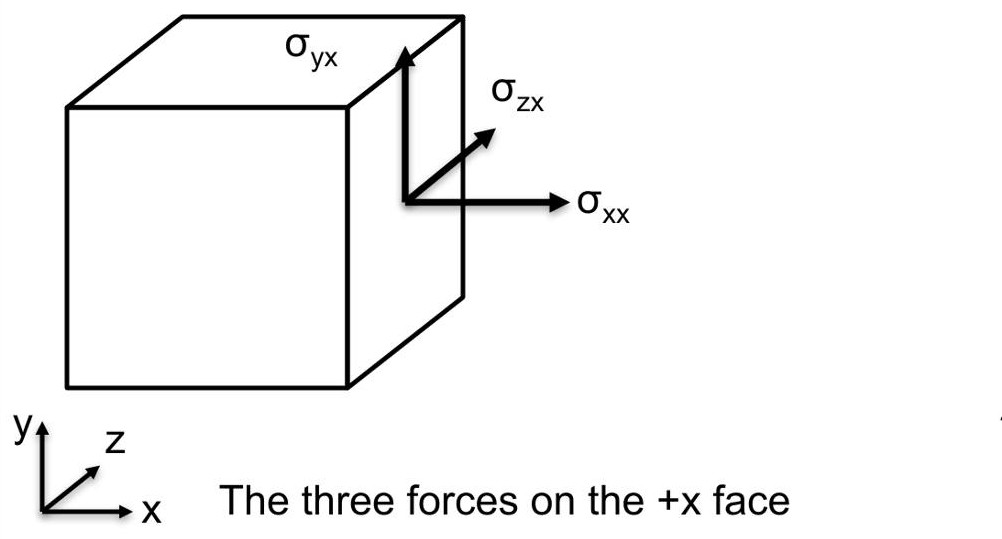
On a small cube, each of the three faces carries a force with three components, so the stress has two indices,

\sigma_{ij} = \frac{\mathrm{d}F_i}{\mathrm{d}A_j} , \qquad \boldsymbol{\sigma} = \begin{pmatrix} \sigma_{xx} & \sigma_{xy} & \sigma_{xz}\\ \sigma_{xy} & \sigma_{yy} & \sigma_{yz}\\ \sigma_{xz} & \sigma_{yz} & \sigma_{zz} \end{pmatrix}.

The first index $i$ is the direction of the force, the second $j$ the direction in which the face points (its outward normal). On the $+x$ face, $\sigma_{xx}$ pulls or pushes along the normal, and $\sigma_{yx}$ and $\sigma_{zx}$ drag along the face. The diagonal entries are tension or compression, the off-diagonal ones shear. If $\sigma_{xy}$ and $\sigma_{yx}$ were different, the shear forces on the $x$ and $y$ faces would twist the cube; with no net torque the tensor is symmetric and has 6 independent entries.

Slide 5: the three forces on the +x face of a cube — Slide 5. The force on the $+x$ face of a small cube has a normal component $\sigma_{xx}$ and two shear components $\sigma_{yx}$ and $\sigma_{zx}$.

Two simple examples close the lecture. Hydrostatic pressure is $\sigma_{ij} = -p\,\delta_{ij}$, with $\delta_{ij}$ the Kronecker delta: the force on every face is normal to it, as in Section 2. And at a free surface normal to $z$, such as the top of an InAs layer grown on GaAs, nothing acts on the surface, no pressure and no shear, so

\sigma_{xz} = \sigma_{yz} = \sigma_{zz} = 0 .

The layer can "breathe" upward until its atoms are at rest. This boundary condition is what determines the vertical expansion of a strained layer in Lecture 23.5.

The force per area on a cut with unit normal $\mathbf{n}$ is the traction $\mathbf{t} = \boldsymbol{\sigma}\, \mathbf{n}$; its $j$-th column is the force on the face pointing along $j$. For the shear load of Section 2:

Code6 lines · cell 11

for name, n in (("+x face", [1, 0, 0]), ("+z face", [0, 0, 1]), ("(x+z)/√2 cut", [1, 0, 1])):
    n = np.array(n, float) / np.linalg.norm(n)
    t = sig_s @ n
    print(f"{name:14s} traction t = σ n = {np.round(t, 3)} GPa, normal part {t @ n:+.3f} GPa, "
          f"shear part {np.linalg.norm(t - (t @ n) * n):.3f} GPa")
print(f"symmetry: σ_xz − σ_zx = {sig_s[0, 2] - sig_s[2, 0]:.1e} GPa")

+x face        traction t = σ n = [-0.  -0.   0.6] GPa, normal part -0.000 GPa, shear part 0.600 GPa
+z face        traction t = σ n = [0.6 0.  0. ] GPa, normal part +0.000 GPa, shear part 0.600 GPa
(x+z)/√2 cut   traction t = σ n = [ 0.424 -0.     0.424] GPa, normal part +0.600 GPa, shear part 0.000 GPa
symmetry: σ_xz − σ_zx = 0.0e+00 GPa

The free-surface condition can be checked on the guiding example of this section. The finite-element model below is a column of GaAs substrate, 5 nm thick, with a 1 nm layer on top, periodic in $x$ and $y$ (an infinitely wide film). The layer is given its own natural lattice constant as an eigenstrain $a_\mathrm{layer}/a_\mathrm{GaAs} - 1$, the strain it would need to fit without forces, and the bottom of the substrate is held. Everything else, including how much the layer expands vertically, is computed. Two layers are compared: InAs, and the alloy In${0.2}$Ga${0.8}$As used in the lectures that follow.

Code32 lines · cell 13

def layer_on_gaas(mat, t_layer=1.0, t_sub=5.0):
    g = Grid(np.linspace(0, 1, 3), np.linspace(0, 1, 3), np.linspace(0, t_sub + t_layer, 61))
    layer = E.Elasticity(g, C_gaas).cell_centers[:, 2] > t_sub
    C_l = E.cubic_stiffness(mat.c11, mat.c12, mat.c44)
    el = E.Elasticity.from_regions(g, [(None, C_gaas, 0.0),
                                       (layer, C_l, mat.lattice_constant / gaas.lattice_constant - 1)],
                                   periodic=(True, True, False))
    el.fix(np.isclose(g.nodes[:, 2], 0), (0, 1, 2), 0.0)
    return layer, el.solve()

zcells = E.Elasticity(Grid(np.linspace(0, 1, 3), np.linspace(0, 1, 3), np.linspace(0, 6, 61)),
                      C_gaas).cell_centers[:, 2]

fig, ax = plt.subplots(figsize=(7, 3.6))
for name, mat, col in (("InAs", kp.material("InAs"), style.OPEN_NEMO),
                       ("In0.2Ga0.8As", kp.material("InGaAs", x=0.2), style.REFERENCE)):
    layer, r_l = layer_on_gaas(mat)
    s = r_l.stress[layer].mean(axis=0)
    print(f"{name:13s} layer stress (GPa): σ_xx = {s[0, 0]:+.3f}, σ_yy = {s[1, 1]:+.3f}, "
          f"σ_zz = {s[2, 2]:+.1e}, σ_xz = {s[0, 2]:+.1e}, σ_yz = {s[1, 2]:+.1e}")
    print(f"{'':13s} in-plane stress = {-s[0, 0] * GPa_in_atm:,.0f} atm of compression; "
          f"substrate |σ| max {np.abs(r_l.stress[~layer]).max():.1e} GPa")
    order = np.argsort(zcells)
    ax.plot(zcells[order], r_l.stress[order, 0, 0], color=col, label=f"{name}: σ_xx = σ_yy")
    ax.plot(zcells[order], r_l.stress[order, 2, 2], color=col, ls=":", label=f"{name}: σ_zz")
ax.axvspan(5, 6, color="0.92", zorder=0)
ax.text(5.1, -3.0, "layer", fontsize=9)
ax.set_xlabel("height z (nm)")
ax.set_ylabel("stress (GPa)")
ax.set_title("Stress in a strained layer on a GaAs substrate")
ax.legend(fontsize=8, loc="lower left")
plt.show()

InAs          layer stress (GPa): σ_xx = -5.686, σ_yy = -5.686, σ_zz = +1.2e-13, σ_xz = -1.2e-15, σ_yz = +1.1e-15
              in-plane stress = 56,118 atm of compression; substrate |σ| max 1.9e-13 GPa
In0.2Ga0.8As  layer stress (GPa): σ_xx = -1.677, σ_yy = -1.677, σ_zz = +1.6e-14, σ_xz = -1.8e-16, σ_yz = +8.1e-17
              in-plane stress = 16,551 atm of compression; substrate |σ| max 2.6e-14 GPa

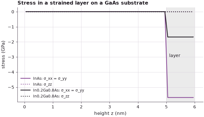
Figure computed by the notebook with open-nemo

In both layers the three stress components that act on the free surface, $\sigma_{zz}$, $\sigma_{xz}$ and $\sigma_{yz}$, vanish to numerical precision, while the in-plane stress is large and compressive: −5.69 GPa (56,118 atm) in InAs and −1.68 GPa (16,551 atm) in In${0.2}$Ga${0.8}$As. The alloy sits inside the slide's range of 0.1–2 GPa; pure InAs on GaAs is far beyond it, which is one way to see why an InAs film gives up after a monolayer or two and forms islands (Lecture 23.1). The thick substrate, wide and held at the bottom, carries no stress in this idealised infinite film.

Summary#

Stress is internal force per area, $\sigma = F/A$; it acts across every imaginary cut. In a pulled GaAs rod (0.1 % strain) it is 0.0862 GPa everywhere, and the force across every cut is the same, 0.345 nN for a 2 nm × 2 nm cross-section; doubling the area doubles the force at the same stress.
1 GPa ≈ 9,869 atm. Strained layers carry 0.1–2 GPa; In${0.2}$Ga${0.8}$As on GaAs has −1.68 GPa, InAs on GaAs −5.69 GPa.
Pressure is $\sigma_{ij} = -p\,\delta_{ij}$ (a 0.5 % uniform compression of GaAs needs 1.18 GPa); a force along a face is shear stress, and a pure shear stress is tension and compression along the diagonals.
The stress tensor $\sigma_{ij} = \mathrm{d}F_i/\mathrm{d}A_j$ is symmetric (6 entries); the traction on a cut is $\boldsymbol{\sigma}\mathbf{n}$; at a free surface normal to $z$, $\sigma_{xz} = \sigma_{yz} = \sigma_{zz} = 0$.
Strain can be seen, stress cannot: the simulation computes the stress from displacements through the elastic constants of Lecture 23.4.

Exercises#

Stretch the rod of Section 1 by 1 % instead of 0.1 %. Does the force scale linearly? Then make the rod from InAs (kp.material("InAs")) and compare the force for the same stretch.
In the shear test, replace the drag along $x$ by a drag along $y$ and confirm that only $\sigma_{yz}$ appears. What happens when you drag along $x$ and $y$ at the same time?
Compute the layer stress of In$x$Ga${1-x}$As on GaAs for $x$ = 0.1 to 0.5 with layer_on_gaas and find the composition at which it exceeds 2 GPa.