

Lecture 1.4
Use of simulation to explain concepts — PN junction to device scaling
In the lecture
- device simulation (TCAD) has been an industrial tool for decades; usability is what makes it a teaching tool
- the PADRE-based apps on nanoHUB (PADRE came from Bell Labs), the ABACUS tool set and their usage
- what a simulator can do that a textbook page cannot: real devices are non-ideal
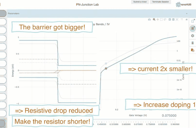
- a pn junction explored interactively: bias changes the barrier and the current grows exponentially; at high bias a resistive drop \(J \propto n\mu\nabla E_F\) limits it; doping 100 times higher makes the barrier bigger; a shorter device recovers the current
- interactive, exploratory learning, and one of the reasons devices are made smaller
In this notebook
we repeat the pn-junction exploration of the slides with a small drift–diffusion simulator: open-nemo's nonlinear Poisson solver for the electrostatic potential and a few lines of numpy for the electron and hole continuity equations (Scharfetter–Gummel discretization, Shockley–Read–Hall recombination, Gummel iteration). We check equilibrium against the depletion approximation and the low-bias current against the Shockley diode equation, then follow the slides: high bias, doping times 100, a shorter device.
Run it on your own machine
The notebook needs open-nemo (Python ≥ 3.10 and a C++20 compiler; BLAS/LAPACK).
git clone https://github.com/denphi/open-nemo.git && cd open-nemo
python3 -m venv .venv && source .venv/bin/activate
pip install -e ".[notebooks]"
jupyter lab From_Atoms_to_Devices/01_introduction/01_4_pn_junction_to_device_scaling.ipynbCode
import numpy as np
import matplotlib.pyplot as plt
import opennemo as nemo
from opennemo.visualization import style

style.use(notebook=True)
from scipy.linalg import solve_banded

props = nemo.structures.properties
T = 300.0
VT = nemo.core.units.KB * T                       # thermal voltage (V)
Q = nemo.core.units.Q                             # elementary charge (C)
EPS0 = nemo.core.units.EPS0                       # vacuum permittivity (F/m)
NC, NV = props.value("Si", "effective_density_conduction"), props.value("Si", "effective_density_valence")
EG, EPS = props.value("Si", "band_gap"), props.value("Si", "eps_static")
NI = np.sqrt(NC * NV) * np.exp(-EG / (2 * VT))   # intrinsic density (cm⁻³)
print(f"Si at 300 K: N_C = {NC:.3g}, N_V = {NV:.3g} cm⁻³, E_g = {EG:.4f} eV, n_i = {NI:.3e} cm⁻³")
Si at 300 K: N_C = 2.86e+19, N_V = 3.1e+19 cm⁻³, E_g = 1.1245 eV, n_i = 1.067e+10 cm⁻³
1. Device simulation for everyone#
Technology computer-aided design (TCAD) tools solve the semiconductor equations for real device geometries; the semiconductor industry has used them for decades. Klimeck's point is about usability: the same physics, wrapped in a simple graphical interface and run in a web browser on nanoHUB, turns a research code into something a student uses on the first day. The PADRE device simulator (from Bell Labs) powers a family of such apps — pn junction, MOSFET, BJT, MOS capacitor — collected in the ABACUS tool set, and they have run hundreds of thousands of simulations.

A textbook page explains the ideal pn junction: the built-in barrier, the depletion region, the exponential current. The question on slide 9 is what a simulator adds — and the answer is that real devices are non-ideal.

2. A drift–diffusion pn diode#
The device is a one-dimensional silicon pn junction, \(L_p\) of p-type (\(N_A\)) and \(L_n\) of n-type (\(N_D\)) material, 6 µm each as in the slides' app. Three equations are solved for the electrostatic potential \(\psi\) and the electron and hole densities \(n\), \(p\):
with \(J_n = q\mu_n n E + qD_n\nabla n\), \(J_p = q\mu_p p E - qD_p\nabla p\) and the
Shockley–Read–Hall recombination \(R = (np - n_i^2)/[\tau(n + n_i) + \tau(p + n_i)]\),
\(\tau = 0.1\) µs. The mobilities follow the doping (Caughey–Thomas). open-nemo's Poisson solves
the first equation by Newton's method for given quasi-Fermi levels; the continuity equations are
linear in \(n\) and \(p\) for a given \(\psi\) and are solved with the Scharfetter–Gummel flux, which is
exact for a constant field between two nodes. The two steps alternate (Gummel iteration) until the
potential stops changing. Ohmic contacts fix \(\psi\), \(n\) and \(p\) at both ends; the bias \(V\) is
applied to the p side.
Code
def caughey_thomas(n, mu_min, mu_max, n_ref, alpha):
    return mu_min + (mu_max - mu_min) / (1 + (n / n_ref) ** alpha)


def bernoulli(z):
    z = np.asarray(z, float)
    small = np.abs(z) < 1e-6
    return np.where(small, 1 - z / 2, z / np.expm1(np.where(small, 1.0, z)))


def tridiag_solve(lo, diag, up, rhs, left, right):
    # banded solve with Dirichlet values at both ends
    a = np.zeros((3, len(diag)))
    a[0, 1:], a[1], a[2, :-1] = up, diag, lo
    a[1, 0], a[0, 1], rhs[0] = 1.0, 0.0, left
    a[1, -1], a[2, -2], rhs[-1] = 1.0, 0.0, right
    return solve_banded((1, 1), a, rhs)


class Diode:
    def __init__(self, na, nd, lp=6000.0, ln=6000.0, dx=5.0, tau=1e-7):
        self.x = np.arange(0.0, lp + ln + dx / 2, dx)           # nm
        self.lp, self.na, self.nd, self.tau = lp, na, nd, tau
        p_side = self.x < lp
        doping = np.where(p_side, na, nd)
        self.mun = caughey_thomas(doping, 68.5, 1414.0, 9.2e16, 0.711)   # cm²/Vs
        self.mup = caughey_thomas(doping, 44.9, 470.5, 2.23e17, 0.719)
        self.poisson = nemo.Poisson(nemo.Grid(self.x), EPS, np.where(p_side, -na, nd), T)
        self.ends = np.zeros(len(self.x), bool)
        self.ends[[0, -1]] = True
        self.psi_p, self.psi_n = -VT * np.log(na / NI), VT * np.log(nd / NI)
        self.psi = np.where(p_side, self.psi_p, self.psi_n)
        self.phin, self.phip = np.zeros(len(self.x)), np.zeros(len(self.x))

    def carriers(self):
        return NI * np.exp((self.psi - self.phin) / VT), NI * np.exp((self.phip - self.psi) / VT)

    def continuity(self, v):
        x, d = self.x * 1e-7, np.diff(self.psi) / VT               # cm; potential step in units of VT
        h = np.diff(x)
        vol = np.zeros(len(x))
        vol[1:] += h / 2
        vol[:-1] += h / 2
        n, p = self.carriers()
        den = self.tau * (n + NI) + self.tau * (p + NI)
        dn = VT * 0.5 * (self.mun[1:] + self.mun[:-1]) / h
        dp = VT * 0.5 * (self.mup[1:] + self.mup[:-1]) / h
        bp, bm = bernoulli(d), bernoulli(-d)
        # electrons: F_{i+1/2} = D/h [n_{i+1} B(d) - n_i B(-d)],  F_{i+1/2} - F_{i-1/2} = R vol
        diag = np.zeros(len(x))
        diag[:-1] -= dn * bm
        diag[1:] -= dn * bp
        n_new = tridiag_solve(dn * bm, diag - p / den * vol, dn * bp, -NI**2 / den * vol,
                              NI * np.exp((self.psi[0] - v) / VT), NI * np.exp(self.psi[-1] / VT))
        # holes: G_{i+1/2} = D/h [p_i B(d) - p_{i+1} B(-d)],  G_{i+1/2} - G_{i-1/2} = -R vol
        diag = np.zeros(len(x))
        diag[:-1] += dp * bp
        diag[1:] += dp * bm
        p_new = tridiag_solve(-dp * bp, diag + n_new / den * vol, -dp * bm, NI**2 / den * vol,
                              NI * np.exp((v - self.psi[0]) / VT), NI * np.exp(-self.psi[-1] / VT))
        self.phin = self.psi - VT * np.log(np.maximum(n_new, 1e-300) / NI)
        self.phip = self.psi + VT * np.log(np.maximum(p_new, 1e-300) / NI)
        jn = Q * dn * (n_new[1:] * bp - n_new[:-1] * bm)
        jp = Q * dp * (p_new[:-1] * bp - p_new[1:] * bm)
        return jn + jp                                             # A/cm² between the nodes

    def solve(self, v, tol=1e-9, max_iter=300):
        self.poisson.set_dirichlet(self.ends, np.where(self.x < self.x.mean(), self.psi_p + v, self.psi_n))
        self.phin[0] = self.phip[0] = v
        for it in range(max_iter):
            n, p = self.carriers()
            new = self.poisson.solve(self.psi, electrons=n, holes=p).potential
            change, self.psi = np.abs(new - self.psi).max(), new
            j = self.continuity(v)
            if change < tol and it > 1:
                break
        return j.mean(), np.ptp(j) / abs(j.mean()), it + 1

    def iv(self, volts):
        return np.array([self.solve(v)[0] for v in volts])
3. Equilibrium: the textbook checks#
At zero bias the depletion approximation predicts the built-in potential, the depletion width and the peak field:
The simulation needs none of these assumptions; the cell compares.
Code
for na, nd in ((1e15, 1e15), (1e17, 1e17)):
    d = Diode(na, nd)
    d.solve(0.0)
    vbi = VT * np.log(na * nd / NI**2)
    w = np.sqrt(2 * EPS * EPS0 * vbi / (Q * 1e6) * (na + nd) / (na * nd)) * 1e9    # nm
    field = np.abs(np.gradient(d.psi, d.x * 1e-7))                                   # V/cm
    n, p = d.carriers()
    rho = p - n + np.where(d.x < d.lp, -na, nd)                    # space charge / q (cm⁻³)
    w_sim = np.trapezoid(np.abs(rho), d.x) / na                    # nm: the depleted width it amounts to
    print(f"N_A = N_D = {na:.0e}: V_bi {np.ptp(d.psi):.4f} V (formula {vbi:.4f});  W = ∫|ρ|dx/qN "
          f"{w_sim:.0f} nm (formula {w:.0f});  E_max {field.max():.3e} V/cm "
          f"(formula {2 * vbi / (w * 1e-7):.3e})")
N_A = N_D = 1e+15: V_bi 0.5919 V (formula 0.5919);  W = ∫|ρ|dx/qN 1192 nm (formula 1248);  E_max 9.025e+03 V/cm (formula 9.487e+03)
N_A = N_D = 1e+17: V_bi 0.8300 V (formula 0.8300);  W = ∫|ρ|dx/qN 143 nm (formula 148);  E_max 1.049e+05 V/cm (formula 1.123e+05)
The built-in potential agrees to the digits printed. The width, measured as the total space charge divided by \(qN\) (the width a fully depleted region would need for the same charge), and the peak field come out a few percent smaller than the formulas, because the real junction is not fully depleted near its edges: free carriers spill about a Debye length into it, which the depletion approximation ignores.
4. Bias changes the barrier: an exponential current#
A forward bias lowers the barrier by \(qV\), and the carriers that cross it (minority carriers on the other side) grow as \(e^{qV/k_BT}\). For neutral regions much shorter than the diffusion length \(\sqrt{D\tau}\) (here about 19 µm for electrons) the Shockley equation is
with \(W_p\), \(W_n\) the widths of the neutral regions.
Code
volts = np.round(np.arange(0.0, 0.901, 0.05), 3)
base = Diode(1e15, 1e15)
j_base = base.iv(volts)

na = nd = 1e15
dn, dp = VT * base.mun[0], VT * base.mup[-1]
vbi = VT * np.log(na * nd / NI**2)
w = np.sqrt(2 * EPS * EPS0 * vbi / (Q * 1e6) * 2 / na) * 1e2                        # cm
wp = wn = 6e-4 - w / 2
j0 = Q * NI**2 * (dn / (na * wp) + dp / (nd * wn))
print(f"D_n = {dn:.1f}, D_p = {dp:.1f} cm²/s, diffusion length sqrt(D_n tau) = "
      f"{np.sqrt(dn * 1e-7) * 1e4:.0f} µm, J_0 = {j0:.3e} A/cm²")
print(" V (V)   J simulation (A/cm²)   J Shockley (A/cm²)   ratio")
for v, j in zip(volts, j_base):
    if v in (0.2, 0.3, 0.4, 0.5, 0.6, 0.7, 0.8, 0.9):
        shockley = j0 * np.expm1(v / VT)
        print(f"{v:5.2f}   {j:18.3e}   {shockley:18.3e}   {j / shockley:6.2f}")
ideality = np.gradient(volts, np.log(np.maximum(j_base, 1e-30))) / VT
print("local ideality factor n = (q/kT) dV/dlnJ at 0.2, 0.5, 0.8 V:",
      np.round(ideality[[4, 10, 16]], 2))
D_n = 35.2, D_p = 11.9 cm²/s, diffusion length sqrt(D_n tau) = 19 µm, J_0 = 1.601e-09 A/cm²
 V (V)   J simulation (A/cm²)   J Shockley (A/cm²)   ratio
 0.20            8.857e-06            3.665e-06     2.42
 0.30            2.214e-04            1.755e-04     1.26
 0.40            8.723e-03            8.397e-03     1.04
 0.50            3.687e-01            4.018e-01     0.92
 0.60            6.934e+00            1.923e+01     0.36
 0.70            3.230e+01            9.202e+02     0.04
 0.80            7.966e+01            4.404e+04     0.00
 0.90            1.484e+02            2.107e+06     0.00
local ideality factor n = (q/kT) dV/dlnJ at 0.2, 0.5, 0.8 V: [1.35 1.1  5.33]
Between 0.4 and 0.5 V the simulation follows the Shockley equation to within 10 %, with a local ideality factor of 1.1: this is the textbook's exponential, and the way a transistor turns on and off. Below that the simulated current is larger (recombination in the depletion region adds a component growing as \(e^{qV/2k_BT}\); the ideality factor is 1.35 at 0.2 V), and from 0.6 V on it falls far below the ideal line (ideality 5.3 at 0.8 V). These are the non-idealities the textbook page mentions in passing; the simulator shows them directly.
5. High bias: the resistive drop#
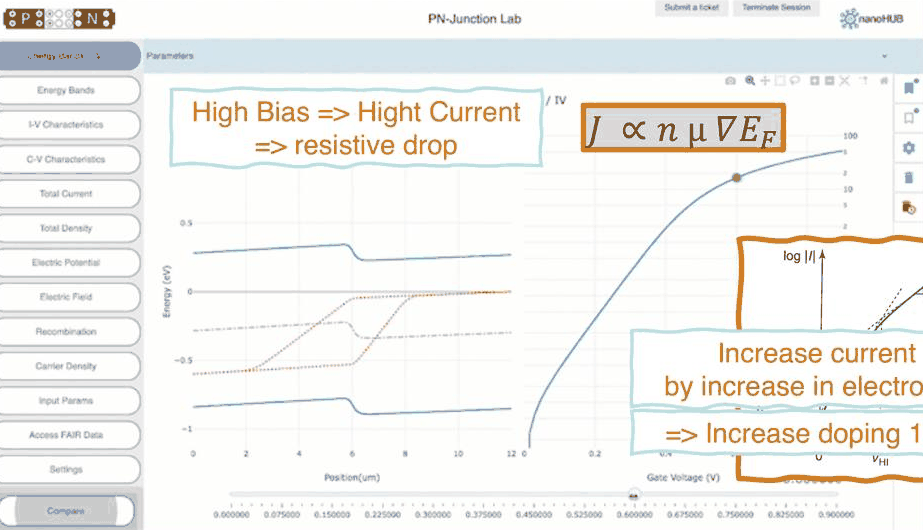
At high current the neutral regions act as resistors: the current density is \(J_n = n\mu_n\nabla E_{Fn}\), so carrying a large \(J\) through a region of modest \(n\) needs a slope of the quasi-Fermi level, a voltage drop that no longer lowers the junction barrier. The band diagram at 0.9 V shows it.
Code
def bands(d, v):
    d.solve(v)
    ec = -d.psi + EG / 2 + VT / 2 * np.log(NV / NC)       # conduction band edge (eV), E_i = -q psi
    return ec, ec - EG, -d.phin, -d.phip


def junction_voltage(d, v):
    # quasi-Fermi level splitting at the junction: n p = n_i² exp(q V_j / kT) there
    d.solve(v)
    k = np.argmin(np.abs(d.x - d.lp))
    return d.phip[k] - d.phin[k]


fig, axes = plt.subplots(1, 2, figsize=(11, 4))
cols = style.sweep(4)
for ax, v in zip(axes, (0.5, 0.9)):
    ec, ev, efn, efp = bands(base, v)
    um = base.x / 1e3
    ax.plot(um, ec, color=style.OPEN_NEMO, label="$E_c$")
    ax.plot(um, ev, color=style.REFERENCE, label="$E_v$")
    ax.plot(um, efn, color=cols[1], ls="--", label="$E_{Fn}$")
    ax.plot(um, efp, color=cols[2], ls=":", label="$E_{Fp}$")
    ax.set(xlabel="position (µm)", ylabel="energy (eV)", title=f"$N_A = N_D = 10^{{15}}$ cm⁻³, V = {v} V")
    ax.legend(fontsize=8)
fig.tight_layout()
for v in (0.5, 0.6, 0.7, 0.8, 0.9):
    vj = junction_voltage(base, v)
    print(f"V = {v}: junction voltage {vj:.3f} V, dropped in the neutral regions {v - vj:.3f} V")
V = 0.5: junction voltage 0.498 V, dropped in the neutral regions 0.002 V
V = 0.6: junction voltage 0.575 V, dropped in the neutral regions 0.025 V
V = 0.7: junction voltage 0.615 V, dropped in the neutral regions 0.085 V
V = 0.8: junction voltage 0.638 V, dropped in the neutral regions 0.162 V
V = 0.9: junction voltage 0.654 V, dropped in the neutral regions 0.246 V
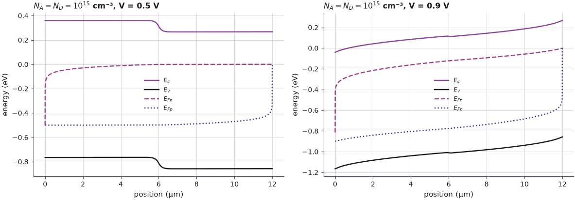
At 0.5 V the majority-carrier quasi-Fermi levels are flat in the neutral regions and split by \(qV\) across the junction: all of the bias lowers the barrier (the minority-carrier quasi-Fermi levels bend back to the majority ones at the contacts, where the diffusing minority carriers recombine). At 0.9 V both quasi-Fermi levels slope across the 6 µm regions, the bands tilt, and only 0.65 V of the 0.9 V reaches the junction; the remaining 0.25 V (already 0.09 V at 0.7 V) is the resistive drop of slide 11. The lightly doped device is also in high injection here: the injected carriers outnumber the doping, and the junction barrier has all but disappeared.
6. Doping 100 times higher — and a shorter device#
The natural fix is more electrons: raise the doping 100 times, to \(10^{17}\) cm⁻³. Slide 13 shows what happens in the app: the resistive drop is reduced, but at the same voltage the current is smaller, because the barrier got bigger (\(V_{bi}\) grows by \(2k_BT\ln 100/q = 0.24\) V) and \(J_0\) falls with \(1/N\). The other fix is to make the resistor shorter.
Code
designs = {"10¹⁵ cm⁻³, 6 + 6 µm": j_base,
           "10¹⁷ cm⁻³, 6 + 6 µm": Diode(1e17, 1e17).iv(volts),
           "10¹⁵ cm⁻³, 1 + 1 µm": Diode(1e15, 1e15, 1000.0, 1000.0, dx=2.0).iv(volts),
           "10¹⁷ cm⁻³, 1 + 1 µm": Diode(1e17, 1e17, 1000.0, 1000.0, dx=2.0).iv(volts)}
print(" V (V)  " + "  ".join(f"{k:>19s}" for k in designs))
for i, v in enumerate(volts):
    if v in (0.3, 0.5, 0.6, 0.7, 0.8, 0.9):
        print(f"{v:5.2f}  " + "  ".join(f"{j[i]:19.3e}" for j in designs.values()))
fig, ax = plt.subplots(figsize=(7, 4.2))
for c, (label, j) in zip(style.sweep(len(designs)), designs.items()):
    ax.semilogy(volts[1:], j[1:], color=c, label=label)
ax.set(xlabel="forward bias V (V)", ylabel="current density J (A/cm²)")
ax.legend(fontsize=8)
fig.tight_layout()
r = designs["10¹⁷ cm⁻³, 6 + 6 µm"] / designs["10¹⁵ cm⁻³, 6 + 6 µm"]
print(f"\ndoping x100 changes J by x{r[volts == 0.5][0]:.3f} at 0.5 V and x{r[volts == 0.9][0]:.2f} at 0.9 V")
 V (V)  10¹⁵ cm⁻³, 6 + 6 µm  10¹⁷ cm⁻³, 6 + 6 µm  10¹⁵ cm⁻³, 1 + 1 µm  10¹⁷ cm⁻³, 1 + 1 µm
 0.30            2.214e-04            3.793e-06            1.608e-03            8.595e-06
 0.50            3.687e-01            2.439e-03            2.448e+00            1.308e-02
 0.60            6.934e+00            1.091e-01            4.257e+01            6.129e-01
 0.70            3.230e+01            5.062e+00            1.946e+02            2.854e+01
 0.80            7.966e+01            1.572e+02            4.527e+02            9.203e+02
 0.90            1.484e+02            1.132e+03            7.723e+02            6.981e+03

doping x100 changes J by x0.007 at 0.5 V and x7.63 at 0.9 V
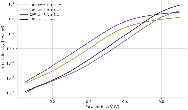
Raising the doping 100 times lowers the current by roughly the factor 100 in \(J_0\) wherever the junction controls it (about 150 times at 0.5 V), and the more conductive device wins only above a crossover between 0.7 and 0.8 V; at 0.9 V it carries 7.6 times more. Shortening both sides from 6 µm to 1 µm helps in both regimes: the diffusion current grows because the minority-carrier gradients get steeper (\(J_0 \propto 1/W\)), and the resistive drop shrinks with the length of the resistor. That is slide 14's conclusion — one of the reasons devices are made smaller. The exploration also shows the method of the course: change one parameter, predict, simulate, and explain the difference.
Summary#
- A drift–diffusion simulator built from open-nemo's nonlinear
Poissonand a Scharfetter–Gummel continuity solve reproduces \(V_{bi}\) exactly and the depletion width and field approximately. - At moderate forward bias (0.4–0.5 V) the current follows the Shockley short-diode equation within 10 % with ideality 1.1; recombination in the junction and the resistive drop make the real diode non-ideal at low and high bias.
- At high bias the quasi-Fermi levels slope in the neutral regions, \(J = n\mu\nabla E_F\), and only part of the bias lowers the barrier.
- Doping 100 times higher raises the barrier and cuts \(J_0\); a shorter device increases the current — one of the reasons for scaling.
Exercises#
- Make the diode asymmetric (\(N_A = 10^{17}\), \(N_D = 10^{15}\) cm⁻³). Which side carries most of the depletion width and which carrier dominates the current? Check against \(J_0\).
- Change \(\tau\) from 0.1 µs to 1 ns. Where in the I–V curve does the change show up, and why?
- Apply a reverse bias of −1 to −5 V and compare the current with the generation current \(qn_iW/2\tau\).
- At which device length does the 10¹⁵ cm⁻³ diode at 0.9 V stop gaining current when made shorter?
Further reading#
- Lecture 1.2: basic device operation
- Si MOS capacitor with Schrödinger–Poisson
- Esaki tunnel diode, a pn junction so heavily doped that tunneling takes over
- open-nemo tools
- R. F. Pierret, Semiconductor Device Fundamentals (Addison-Wesley, 1996), chapter 6.
- J. A. del Alamo, Integrated Microelectronic Devices (Pearson, 2017).
- D. L. Scharfetter and H. K. Gummel, IEEE Trans. Electron Devices 16, 64 (1969).
- PN Junction Lab on nanoHUB: nanohub.org/tools/pntoy; ABACUS: nanohub.org/tools/abacus.