Lecture 22.2

Optical matrix elements — allowed and forbidden transitions

In the lecture

The box states relabelled from $n = 0$ with the origin in the middle of the box, so that even $n$ are even functions and odd $n$ odd functions of $x$.
The dipole integral $\int\psi_i\,x\,\psi_f\,dx$ built graphically, factor by factor, for the transitions 0 → 1 and 1 → 2 (allowed) and 0 → 2, 0 → 4 and 1 → 3 (forbidden).
The table of all transitions between the lowest eight states: a checkerboard in which half of the transitions are dark.
The general proof by symmetry: the integral of an odd function over a symmetric interval vanishes, so only transitions between states of opposite parity are allowed, whatever the symmetric potential.
Upward (absorption) and downward (emission) transitions obey the same rule.

In this notebook

you compute the states of the centred box with open-nemo, check their parity, draw the integrands of the lecture's five example transitions and integrate them, build the 8 × 8 table of dipole matrix elements (and check it against the library's velocity operator), verify the half-domain formula of the proof, show that the same selection rule holds for a finite well, a harmonic well and a double well, and watch the forbidden transitions light up when an asymmetric step or a static field breaks the symmetry.

Run the notebookEvery number and figure on this page comes from it. Change it, rerun it, take it further.

Download .ipynb View on GitHub

Run it on your own machine

The notebook needs open-nemo (Python ≥ 3.10 and a C++20 compiler; BLAS/LAPACK).

git clone https://github.com/denphi/open-nemo.git && cd open-nemo
python3 -m venv .venv && source .venv/bin/activate
pip install -e ".[notebooks]"
jupyter lab From_Atoms_to_Devices/08_optical_matrix_elements/22_2_allowed_and_forbidden_transitions.ipynb

Code9 lines · cell 1

import numpy as np
import matplotlib.pyplot as plt
from scipy.linalg import eigh_tridiagonal
import opennemo as nemo
from opennemo.core import units
from opennemo.simulations import optics
from opennemo.visualization import style

style.use(notebook=True)

1. Labelling the states from n = 0: even and odd parity#

Lecture 22.1 showed that for ordinary light the box states stay the unperturbed sines and that the strength of a transition $i \to f$ is the dipole matrix element

\mu_{if} = e\int dx\;\psi_i(x)\,x\,\psi_f(x).

To see which of these integrals vanish, the lecture moves the origin to the middle of the box, so the walls are at $x = \pm L/2$, and counts the states from $n = 0$:

\psi_n(x) = \sqrt{\frac{2}{L}}\,\sin\frac{(n+1)\pi\,(x + L/2)}{L},\qquad E_n = \frac{\hbar^2\pi^2 (n+1)^2}{2m^*L^2},\qquad n = 0, 1, 2, \dots

With this choice the parity of a state follows its label. The states with even $n$ (the ground state $n = 0$, the three-lobed $n = 2$) are even functions, $E(x) = E(-x)$; the states with odd $n$ ($n = 1$, $n = 3$) are odd, $O(x) = -O(-x)$. Parity is a property of the wave function, not of the labels: the shift of origin only makes it visible. We compute the states of a centred 10 nm GaAs box with open-nemo's effective-mass model and measure the parity of each as $P_n = \int\psi_n(x)\, \psi_n(-x)\,dx$, which is $+1$ for an even and $-1$ for an odd state.

Code29 lines · cell 3

M, L, DX = 0.067, 10.0, 0.02          # GaAs electron mass (m0), box width and grid spacing (nm)
H2M0 = units.HBAR2_2M0
gaas = nemo.structures.materials.EffectiveMassMaterial("GaAs", M, 12.9)


def solve(dev, potential=0.0, num=8):
    """Lowest `num` states of a closed Heterostructure1D (hard walls one spacing beyond its end sites)
    with an extra potential energy (eV per site): centred x (nm), energies (eV), ψ (1/√nm, columns)."""
    dx = dev.spacing
    x = dev.x - dev.x.mean()            # the grid is symmetric about the centre of the device
    h = dev.hamiltonian.sparse.matrices[0].real
    e, psi = eigh_tridiagonal(h.diagonal() + potential, h.diagonal(1), select="i",
                              select_range=(0, num - 1))
    psi = psi / np.sqrt(dx)
    psi *= np.sign(psi[np.argmax(np.abs(psi), axis=0), np.arange(num)])   # largest lobe positive
    return x, e, psi


def dipoles(x, psi, dx=DX):
    return psi.T @ (x[:, None] * psi) * dx    # <ψi|x|ψf> (nm), all pairs


box = nemo.Heterostructure1D([nemo.Layer(gaas, L - DX)], spacing=DX)   # a box exactly L wide
x, e, psi = solve(box)
parity = np.sum(psi * psi[::-1], axis=0) * DX                           # ∫ ψ(x) ψ(−x) dx
print("n   E_n (meV)   ħ²π²(n+1)²/2m*L²   parity")
for n in range(8):
    exact = H2M0 * np.pi**2 * (n + 1) ** 2 / (M * L**2)
    print(f"{n}   {1e3 * e[n]:8.2f}   {1e3 * exact:12.2f}       {parity[n]:+.6f}")

n   E_n (meV)   ħ²π²(n+1)²/2m*L²   parity
0      56.12          56.12       +1.000000
1     224.49         224.50       -1.000000
2     505.10         505.12       +1.000000
3     897.94         897.98       -1.000000
4    1402.98        1403.10       +1.000000
5    2020.22        2020.46       -1.000000
6    2749.63        2750.07       +1.000000
7    3591.17        3591.93       -1.000000

Code13 lines · cell 4

fig, axs = plt.subplots(4, 1, figsize=(5.2, 6.0), sharex=True)
for ax, n in zip(axs, (3, 2, 1, 0)):
    c = style.sweep(2)[n % 2]
    ax.plot(x, psi[:, n], color=c, lw=1.8)
    ax.axhline(0, color=style.CONTEXT, lw=0.6)
    ax.axvline(0, color=style.CONTEXT, lw=0.6)
    kind = "even: E(x) = E(−x)" if n % 2 == 0 else "odd: O(x) = −O(−x)"
    ax.text(0.99, 0.80, f"n = {n}, {kind}", transform=ax.transAxes, ha="right", fontsize=8)
    ax.set(yticks=[], xlim=(-L / 2, L / 2))
    ax.grid(False)
axs[-1].set(xlabel="x (nm), walls at ±L/2")
axs[0].set_title("states of the centred 10 nm box", fontsize=10)
fig.tight_layout()

Figure computed by the notebook with open-nemo

The parities come out $\pm 1$ to machine precision, alternating with $n$.

2. Building the integral graphically#

The lecture then evaluates the integral without computing it, by building the integrand $\psi_i \cdot x \cdot \psi_f$ factor by factor. For 0 → 1: first multiply the final state, the odd $\psi_1$, by the odd, linearly rising $x$. The product of two odd functions is even, and here even positive everywhere. Multiplied by the even, single-lobed $\psi_0$ it stays even and positive, so its integral is finite: the transition is allowed.

Slide 8: the integrand of the 0 → 1 transition — Slide 8: x times the odd ψ₁ is even; times the even ψ₀ the integrand is even and positive, the integral finite: an allowed transition.

The same steps for 1 → 2: $x\,\psi_2$ is odd (odd times even), and times the odd $\psi_1$ the integrand is even: allowed. For 0 → 2, $x\,\psi_2$ is odd, and times the even $\psi_0$ the whole integrand is odd: its positive and negative halves cancel exactly and the integral is zero, a forbidden transition. The same happens for 0 → 4 (even to even) and for 1 → 3, where $x\,\psi_3$ is even and the odd $\psi_1$ makes the integrand odd.

Slide 11: the integrand of the 0 → 2 transition — Slide 11: for 0 → 2 the product ψ₀ · x · ψ₂ is an odd function, its integral zero: forbidden.

We draw the three factors and the integrand of the five transitions of the lecture with the open-nemo states, and integrate:

Code28 lines · cell 6

pairs = [(0, 1), (1, 2), (0, 2), (0, 4), (1, 3)]
fig, axs = plt.subplots(len(pairs), 3, figsize=(10, 8.4), sharex=True)
for row, (i, f) in zip(axs, pairs):
    xf = x * psi[:, f]
    integrand = psi[:, i] * xf
    mu = np.sum(integrand) * DX
    allowed = abs(mu) > 1e-8 * L
    row[0].plot(x, psi[:, i], color=style.sweep(2)[i % 2])
    row[0].set_ylabel(f"{i} → {f}", rotation=0, labelpad=18, fontsize=10)
    row[1].plot(x, xf, color=style.sweep(2)[(f + 1) % 2])
    row[2].fill_between(x, integrand, where=integrand > 0, color=style.OPEN_NEMO, alpha=0.5, lw=0)
    row[2].fill_between(x, integrand, where=integrand < 0, color=style.CONTEXT, alpha=0.6, lw=0)
    row[2].plot(x, integrand, color="k", lw=0.8)
    verdict = "allowed" if allowed else "forbidden"
    row[2].text(0.98, 0.84, f"∫ = {mu:+.4f} nm: {verdict}", transform=row[2].transAxes, ha="right",
                fontsize=8, bbox=dict(fc="w", ec="none", alpha=0.85))
    for ax in row:
        ax.axhline(0, color=style.CONTEXT, lw=0.5)
        ax.axvline(0, color=style.CONTEXT, lw=0.5)
        ax.set(yticks=[], xlim=(-L / 2, L / 2))
        ax.grid(False)
    print(f"{i} -> {f}: parity {'even' if i % 2 == 0 else 'odd'} -> {'even' if f % 2 == 0 else 'odd'}, "
          f"<ψ{i}|x|ψ{f}> = {mu:+.3e} nm  ({verdict})")
for ax, t in zip(axs[0], ("initial state ψᵢ", "x · ψ_f", "integrand ψᵢ · x · ψ_f")):
    ax.set_title(t, fontsize=10)
for ax in axs[-1]:
    ax.set_xlabel("x (nm)")
fig.tight_layout()

0 -> 1: parity even -> odd, <ψ0|x|ψ1> = +1.801e+00 nm  (allowed)
1 -> 2: parity odd -> even, <ψ1|x|ψ2> = -1.945e+00 nm  (allowed)
0 -> 2: parity even -> even, <ψ0|x|ψ2> = +1.393e-13 nm  (forbidden)
0 -> 4: parity even -> even, <ψ0|x|ψ4> = +7.674e-15 nm  (forbidden)
1 -> 3: parity odd -> odd, <ψ1|x|ψ3> = -9.990e-14 nm  (forbidden)

The allowed integrands are even and of one dominant sign; the forbidden ones are odd and their integrals vanish to round-off ($10^{-13}$ nm and below, against 1.80 and 1.95 nm for the allowed ones).

3. The table of allowed and forbidden transitions#

Collecting the five cases: even → odd and odd → even are allowed, even → even and odd → odd are forbidden. The lecture reorders all transitions between the first states into a table with the initial state $i$ as the row and the final state $f$ as the column. It is a checkerboard: from $i = 0$ the transitions to $f = 1, 3, 5$ are allowed and those to $f = 2, 4, 6$ forbidden, from $i = 1$ the reverse, and so on, with no entry on the diagonal ($i = f$ is no transition).

Slide 17: the checkerboard of allowed (green) and forbidden (yellow) transitions — Slide 17: allowed transitions (green) and forbidden transitions (yellow) for i = 0 … 3 and f = 0 … 6.

We compute the full 8 × 8 table of $|\langle\psi_i|x|\psi_f\rangle|$ from the open-nemo states. As an independent check we take the library's optics module, which builds the velocity operator $\hbar v = i[H, x]$ from the Hamiltonian (optics.velocity) and its matrix elements between the eigenstates (optics.transitions). Between eigenstates $\langle i|\hbar v|f\rangle = i(E_i - E_f) \langle i|x|f\rangle$, so the two must give the same table.

Code17 lines · cell 8

X = dipoles(x, psi)
h = box.hamiltonian.sparse.matrices[0]
tr = optics.transitions(h, optics.velocity(box.hamiltonian), (-1.0, -0.5), num_conduction=8,
                        num_valence=0)
de = tr["energies"][None, :] - tr["energies"][:, None]
with np.errstate(divide="ignore", invalid="ignore"):
    X_v = np.where(np.eye(8, dtype=bool), 0.0, np.sqrt(tr["matrix"][0]) / np.abs(de))
off = ~np.eye(8, dtype=bool)
print("|<ψi|x|ψf>| (nm), rows i, columns f")
print("     " + "".join(f"{f:8d}" for f in range(8)))
for i in range(8):
    print(f"{i:3d}  " + "".join("       ·" if i == f else f"{abs(X[i, f]):8.4f}" for f in range(8)))
print(f"largest difference to the velocity-operator route: {np.abs(np.abs(X) - X_v)[off].max():.1e} nm")
allowed = (np.abs(X) > 1e-6 * L) & off
up = np.triu(allowed).sum()
print(f"allowed: {allowed.sum()} of {off.sum()} ordered pairs ({up} up, {allowed.sum() - up} down)")
assert np.array_equal(allowed, ((np.add.outer(range(8), range(8)) % 2) == 1))

|<ψi|x|ψf>| (nm), rows i, columns f
            0       1       2       3       4       5       6       7
  0         ·  1.8013  0.0000  0.1441  0.0000  0.0397  0.0000  0.0163
  1    1.8013       ·  1.9454  0.0000  0.1838  0.0000  0.0560  0.0000
  2    0.0000  1.9454       ·  1.9851  0.0000  0.2001  0.0000  0.0643
  3    0.1441  0.0000  1.9851       ·  2.0014  0.0000  0.2084  0.0000
  4    0.0000  0.1838  0.0000  2.0014       ·  2.0097  0.0000  0.2132
  5    0.0397  0.0000  0.2001  0.0000  2.0097       ·  2.0144  0.0000
  6    0.0000  0.0560  0.0000  0.2084  0.0000  2.0144       ·  2.0174
  7    0.0163  0.0000  0.0643  0.0000  0.2132  0.0000  2.0174       ·
largest difference to the velocity-operator route: 1.3e-13 nm
allowed: 32 of 56 ordered pairs (16 up, 16 down)

Code18 lines · cell 9

fig, ax = plt.subplots(figsize=(5.6, 4.8))
shown = np.where(off, np.abs(X) / L, np.nan)
im = ax.imshow(shown, cmap=style.MAGNITUDE, vmin=0, origin="upper")
for i in range(8):
    for f in range(8):
        if i == f:
            label = "·"
        elif allowed[i, f]:
            label = "U" if f > i else "D"
        else:
            label = "–"
        ax.text(f, i, label, ha="center", va="center", fontsize=9,
                color="w" if np.nan_to_num(shown[i, f]) > 0.1 else "k")
ax.set(xticks=range(8), yticks=range(8), xlabel="final state f", ylabel="initial state i",
       title="|⟨ψᵢ|x|ψ_f⟩| / L: U up, D down, – forbidden")
ax.grid(False)
fig.colorbar(im, ax=ax, label="|⟨ψᵢ|x|ψ_f⟩| / L")
fig.tight_layout()

The open-nemo table is the lecture's checkerboard: of the 56 ordered pairs of distinct states, the 32 with $f - i$ odd are allowed (16 absorptions "U" above the diagonal, 16 emissions "D" below it) and the 24 with $f - i$ even are dark. The velocity-operator route of the library gives the same numbers to round-off. The table also shows what lecture 22.3 derives: the strongest elements sit next to the diagonal and they fade as $f$ and $i$ move apart.

4. The general proof by symmetry#

The graphical argument used sines, but the lecture generalizes it with two facts about integrals over a symmetric interval. Splitting the interval at $0$ and substituting $x \to -x$ in the left half:

\int_{-L/2}^{L/2} E(x)\,dx = \int_{-L/2}^{0} E(-x)\,dx + \int_0^{L/2} E(x)\,dx = 2\int_0^{L/2}E(x)\,dx, \qquad \int_{-L/2}^{L/2} O(x)\,dx = -\int_0^{L/2}O(x)\,dx + \int_0^{L/2}O(x)\,dx = 0 .

Apply them to the three classes of matrix elements, with $O$ an odd and $E$ an even state:

odd → even: $O(x)\,x\,E(x)$ is even, so $\mu_{oe} = 2e\int_0^{L/2} O(x)\,x\,E(x)\,dx \ne 0$ in general: allowed, and it can be computed on half the domain;
odd → odd: $O(x)\,x\,O(x)$ is odd, so $\mu_{oo} = 0$: forbidden;
even → even: $E(x)\,x\,E(x)$ is odd, so $\mu_{ee} = 0$: forbidden.

Nothing in the proof refers to sines. It needs only that the potential is symmetric, $V(x) = V(-x)$, so that every (non-degenerate) eigenstate is either even or odd. First the half-domain formula, for the odd → even transition 1 → 2:

Code6 lines · cell 11

right = x > 0
half = 2 * np.sum(psi[right, 1] * x[right] * psi[right, 2]) * DX
print(f"<ψ1|x|ψ2> over the whole box: {X[1, 2]:+.6f} nm;  2 × ∫ over 0 < x < L/2: {half:+.6f} nm")
print(f"<ψ1|x|ψ3> over the whole box: {X[1, 3]:+.1e} nm;  "
      f"left and right halves: {np.sum((psi[:, 1] * x * psi[:, 3])[~right]) * DX:+.4f}, "
      f"{np.sum((psi[:, 1] * x * psi[:, 3])[right]) * DX:+.4f} nm")

<ψ1|x|ψ2> over the whole box: -1.945367 nm;  2 × ∫ over 0 < x < L/2: -1.945367 nm
<ψ1|x|ψ3> over the whole box: -9.9e-14 nm;  left and right halves: +0.4503, -0.4503 nm

Now the claim that the rule holds for any symmetric potential. We build four symmetric structures with open-nemo and one asymmetric one, and compute their tables:

the infinite box of the lecture;
a finite well: 10 nm of GaAs between Al${0.3}$Ga${0.7}$As barriers (taken here as a 0.25 eV step and $m^* = 0.092\,m_0$; the states above the barrier top are box states of the whole structure);
a harmonic well, $V = \tfrac12 m^*\omega_0^2 x^2$ with $\hbar\omega_0 = 30$ meV, in a 60 nm GaAs box;
a double well: two 6 nm GaAs wells separated by a 2 nm barrier of 0.25 eV;
an asymmetric step well: a 10 nm box whose right half is raised by 0.1 eV.

Code22 lines · cell 13

algaas = nemo.structures.materials.EffectiveMassMaterial("AlGaAs", 0.092, 12.2, conduction_band_edge=0.25)
Layer = nemo.Layer
structures = {}
structures["infinite box"] = (box, 0.0)
structures["finite well"] = (nemo.Heterostructure1D([Layer(algaas, 8), Layer(gaas, L), Layer(algaas, 8)],
                                                    spacing=DX), 0.0)
wide = nemo.Heterostructure1D([Layer(gaas, 60 - DX)], spacing=DX)
xw = wide.x - wide.x.mean()
hw0 = 0.030                                                # ħω0 (eV)
structures["harmonic well"] = (wide, hw0**2 / (4 * H2M0 / M) * xw**2)   # ½ m*ω0² x² in eV
structures["double well"] = (nemo.Heterostructure1D([Layer(algaas, 6), Layer(gaas, 6), Layer(algaas, 2),
                                                     Layer(gaas, 6), Layer(algaas, 6)], spacing=DX), 0.0)
structures["asymmetric step"] = (box, np.where(x > 0, 0.1, 0.0))

tables = {}
for name, (dev, pot) in structures.items():
    xs, es, ps = solve(dev, pot)
    par = np.sum(ps * ps[::-1], axis=0) * DX
    tables[name] = np.abs(dipoles(xs, ps, dev.spacing))
    even_even = tables[name][(np.add.outer(range(8), range(8)) % 2) == 0].max()
    print(f"{name:16s} parities {' '.join(f'{p:+.2f}' for p in par)}   "
          f"largest |x| between equal parities: {even_even:.1e} nm")

infinite box     parities +1.00 -1.00 +1.00 -1.00 +1.00 -1.00 +1.00 -1.00   largest |x| between equal parities: 3.3e-13 nm
finite well      parities +1.00 -1.00 +1.00 -1.00 +1.00 -1.00 +1.00 -1.00   largest |x| between equal parities: 9.1e-12 nm
harmonic well    parities +1.00 -1.00 +1.00 -1.00 +1.00 -1.00 +1.00 -1.00   largest |x| between equal parities: 4.6e-12 nm
double well      parities +1.00 -1.00 +1.00 -1.00 +1.00 -1.00 +1.00 -1.00   largest |x| between equal parities: 7.2e-12 nm
asymmetric step  parities +0.89 -0.88 +0.97 -0.98 +0.99 -0.99 +0.99 -0.99   largest |x| between equal parities: 8.2e-01 nm

Code12 lines · cell 14

from matplotlib.colors import LogNorm

fig, axs = plt.subplots(1, 5, figsize=(14, 3.3))
diag = np.eye(8, dtype=bool)
for ax, (name, t) in zip(axs, tables.items()):
    t = np.where(diag, np.nan, np.maximum(t / t[~diag].max(), 1e-4))   # zeros shown at the floor
    im = ax.imshow(t, cmap=style.MAGNITUDE, norm=LogNorm(1e-4, 1))
    ax.set(xticks=range(0, 8, 2), yticks=range(0, 8, 2), title=name, xlabel="f")
    ax.grid(False)
axs[0].set_ylabel("i")
fig.colorbar(im, ax=axs, shrink=0.8, label="relative |⟨ψᵢ|x|ψ_f⟩|")
fig.suptitle("|⟨ψᵢ|x|ψ_f⟩| relative to the largest element of each structure (log scale)", fontsize=10)

Text(0.5, 0.98, '|⟨ψᵢ|x|ψ_f⟩| relative to the largest element of each structure (log scale)')

All four symmetric structures have states of alternating parity and the same checkerboard: the matrix elements between states of equal parity vanish to round-off ($10^{-11}$ nm at most). The harmonic well is stricter still: its only non-zero elements are the neighbours, $f = i \pm 1$, because $x$ is a sum of a raising and a lowering operator for the oscillator (the one exception, 0.002 nm between states 4 and 7, comes from the walls of the 60 nm box, which the highest states begin to feel). The symmetry argument says which transitions must vanish; a particular potential can forbid more. In the double well the two lowest states are the even (bonding) and odd (antibonding) combinations of the ground states of the two wells, and their element $|x_{01}| = 3.99$ nm is about half the 8 nm distance between the well centres: the transition moves charge from one well to the other. The asymmetric step has no parity (its states' $P_n$ are 0.88 to 0.99 in magnitude, not 1), and every element of the table is finite, up to 0.82 nm between states of "equal" parity.

5. Up and down transitions#

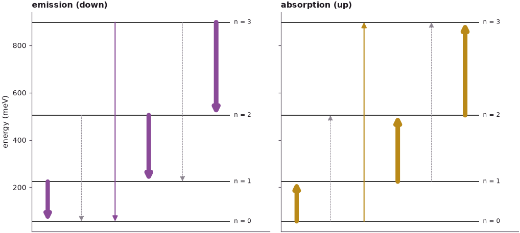
The same table serves both directions. $|\mu_{if}| = |\mu_{fi}|$, so a transition allowed upward (absorption of a photon, "U" in the table) is allowed downward (emission, "D") with the same strength. In the one-dimensional box only half of all transitions are optically active; the others are dark — "verboten" in the German of early quantum mechanics, which is where the term forbidden transition comes from.

Slide 23: emission (red) and absorption (blue) between the box states, and the U/D table — Slide 23: downward (red) and upward (blue) transitions between the levels n = 0 … 3, the forbidden ones in grey, and the table of up (U) and down (D) transitions.

We draw the same diagram from the open-nemo levels, with each allowed arrow as wide as its matrix element:

Code23 lines · cell 16

fig, axs = plt.subplots(1, 2, figsize=(9.5, 4.4), sharey=True)
for ax, up in zip(axs, (False, True)):
    for n in range(4):
        ax.hlines(1e3 * e[n], 0, 1, color="k", lw=1)
        ax.text(1.02, 1e3 * e[n], f"n = {n}", va="center", fontsize=8)
    slot = 0
    for i in range(4):
        for f in range(i + 1, 4):
            pos = 0.08 + 0.85 * slot / 5
            slot += 1
            lo, hi = 1e3 * e[i], 1e3 * e[f]
            start, end = (lo, hi) if up else (hi, lo)
            if allowed[i, f]:
                colour = style.sweep(2)[0] if up else style.OPEN_NEMO
                props = dict(arrowstyle="-|>", color=colour, lw=1 + 2.5 * abs(X[i, f]))
            else:
                props = dict(arrowstyle="-|>", color=style.CONTEXT, lw=0.8, ls=":")
            ax.annotate("", (pos, end), (pos, start),
                        arrowprops=dict(props, shrinkA=0, shrinkB=0, mutation_scale=14))
    ax.set(xlim=(0, 1.2), xticks=[], title="absorption (up)" if up else "emission (down)")
    ax.grid(False)
axs[0].set_ylabel("energy (meV)")
fig.tight_layout()

6. Exploration: breaking the symmetry with a field#

The selection rule is exact only as long as the potential is symmetric. A static electric field across the well (from a gate, a built-in polarization field or a bias) tilts the floor as in lecture 22.1 and removes the symmetry: the states lose their parity and the forbidden transitions acquire a strength. To first order in the field $\mathcal{E}$ the states mix with their neighbours of opposite parity, so the forbidden element 0 → 2 grows linearly with $\mathcal{E}$ while the allowed 0 → 1 hardly changes:

Code20 lines · cell 18

fields = np.linspace(0, 20, 21) * 1e-3                       # V/nm (0 … 20 MV/m)
x02, x01, x13 = [], [], []
for F in fields:
    _, _, pf = solve(box, F * x)
    xf = np.abs(dipoles(x, pf))
    x02.append(xf[0, 2]), x01.append(xf[0, 1]), x13.append(xf[1, 3])
x02, x01, x13 = map(np.array, (x02, x01, x13))
fig, ax = plt.subplots(figsize=(6.5, 4))
ax.plot(fields * 1e3, x01 / L, color=style.OPEN_NEMO, label="0 → 1 (allowed)")
ax.plot(fields * 1e3, x02 / L, color=style.sweep(2)[0], label="0 → 2 (forbidden at ℰ = 0)")
ax.plot(fields * 1e3, x13 / L, "--", color=style.sweep(2)[1], label="1 → 3 (forbidden at ℰ = 0)")
ax.set(xlabel="static field ℰ (MV/m)", ylabel="|⟨ψᵢ|x|ψ_f⟩| / L",
       title="10 nm GaAs box in a static field")
ax.legend(fontsize=8, frameon=False)
fig.tight_layout()
k = 5
print(f"at {fields[k] * 1e3:.0f} MV/m: |x02| = {x02[k]:.4f} nm, |x13| = {x13[k]:.4f} nm, "
      f"|x01| = {x01[k]:.4f} nm (field-free {x01[0]:.4f} nm)")
print(f"at {fields[-1] * 1e3:.0f} MV/m: |x02| = {x02[-1]:.4f} nm, |x01| = {x01[-1]:.4f} nm;  "
      f"|x02| / ℰ at 5 and 20 MV/m: {x02[k] / fields[k]:.1f}, {x02[-1] / fields[-1]:.1f} nm²/V")

at 5 MV/m: |x02| = 0.0468 nm, |x13| = 0.0157 nm, |x01| = 1.7959 nm (field-free 1.8013 nm)
at 20 MV/m: |x02| = 0.1752 nm, |x01| = 1.7236 nm;  |x02| / ℰ at 5 and 20 MV/m: 9.4, 8.8 nm²/V

At 5 MV/m (a third of the Airy threshold of lecture 22.1) the formerly forbidden 0 → 2 element is 0.047 nm, 3 % of the allowed 0 → 1 element (and its square, which sets the rate, 0.07 %); it grows nearly linearly, to 0.18 nm at 20 MV/m, while the allowed 0 → 1 element drops by only 4 %, from 1.80 to 1.72 nm. The 1 → 3 element grows too, but more slowly (0.016 nm at 5 MV/m). In quantum wells under bias this is how forbidden transitions such as e1–hh2 appear in absorption spectra.

Summary#

With the origin in the middle of the box and the states counted from $n = 0$, even $n$ are even and odd $n$ odd functions; open-nemo's states have parities $\pm1$ to machine precision.
$x$ is odd, so $\psi_i\,x\,\psi_f$ is even (finite integral, allowed) when $\psi_i$ and $\psi_f$ have opposite parity, and odd (zero integral, forbidden) when they have the same parity.
The 8 × 8 table of $|\langle\psi_i|x|\psi_f\rangle|$ is a checkerboard: 32 of the 56 transitions are allowed (16 up, 16 down), and the library's velocity operator reproduces every element.
The proof uses only the symmetry of the potential: a finite well, a harmonic well and a double well give the same checkerboard (the harmonic well an even sparser table, $f = i \pm 1$), while an asymmetric step or a static field makes the forbidden transitions weakly allowed.

Exercises#

Compute the half-domain formula $\mu_{oe} = 2e\int_0^{L/2}O\,x\,E\,dx$ for 0 → 3 and 2 → 5 and compare with the full-domain integrals.
In the finite well, vary the barrier height from 0.05 eV to 1 eV. Which states stay bound, and does the checkerboard survive for all of them?
In the harmonic well, check numerically that $|\langle\psi_n|x|\psi_{n+1}\rangle| = \sqrt{(n+1)/2}\, \ell$ with $\ell = \sqrt{\hbar/(m^*\omega_0)}$, and that the elements with $|f - i| = 3$ vanish.
Repeat the field sweep for a 5 nm and a 20 nm box. How does $|x_{02}|/\mathcal{E}$ at small field scale with $L$? (Perturbation theory gives a power law.)