Lecture 21.1

NEMO 3-D — multi-scale by design

Lecture page Video Slides

In the lecture

The plan of lecture 21: strain from balls and springs (21.2), the sp3d5s* tight-binding basis (21.3), Lanczos eigenvalues (21.4), parallel computing (21.5) and validation (21.6).
Why nanostructures need an atom-by-atom, local-orbital description, but not an ab initio one: semiconductor bonds are stable, the structures are finite, and they contain millions of atoms.
The NEMO 3-D chain: geometry → atomistic relaxation (valence force field) → strain and piezoelectric potential → tight-binding Hamiltonian → single-particle states → optical and transport properties → many-body interactions.
End-to-end runs of up to 52 million atoms, a $(101\ \mathrm{nm})^3$ cube, whose time grows linearly with the number of atoms.
The InGaAs alloy is not a crystal with an average bond: its In–As and Ga–As bonds stay close to their own lengths (a bimodal distribution).

In this notebook

Count the atoms and Hamiltonian rows of NEMO 3-D-sized domains.
Run the whole NEMO 3-D chain on a small InAs pyramid in GaAs with open-nemo — geometry, Keating relaxation, strain, strained tight-binding Hamiltonian, Lanczos eigenvalues — and time each step.
Relax random In$x$Ga${1-x}$As supercells and show the bimodal bond lengths against Vegard's law.

Run the notebookEvery number and figure on this page comes from it. Change it, rerun it, take it further.

Download .ipynb View on GitHub

Run it on your own machine

The notebook needs open-nemo (Python ≥ 3.10 and a C++20 compiler; BLAS/LAPACK).

git clone https://github.com/denphi/open-nemo.git && cd open-nemo
python3 -m venv .venv && source .venv/bin/activate
pip install -e ".[notebooks]"
jupyter lab From_Atoms_to_Devices/07_quantum_dots_and_nemo3d/21_1_nemo3d_multiscale_by_design.ipynb

Code11 lines · cell 1

import time
import numpy as np
import matplotlib.pyplot as plt
import opennemo as nemo
from opennemo.visualization import style
from opennemo.models import mechanics as M
from opennemo.structures.structure import Structure, bulk, random_alloy, supercell
from opennemo.solvers.eigen import lanczos_window_eigenstates
from scipy.spatial import cKDTree

style.use(notebook=True)

1. Why an atomistic, local-orbital, non-ab-initio model#

Klimeck lists the requirements of nanoscale device simulation and the choice each one forces:

The structures cannot be described as bulk or "jellium": the atoms are countable, so the description must be atom by atom — with pseudopotentials or with local orbitals.
The devices have finite extent and are not periodic, which favours local orbitals over plane waves (plane waves are awkward in heterostructures).
The bonds of the semiconductors of interest are stable: nobody wants a device with dangling bonds ("pretty much an unstable device", in his words, said tongue in cheek). There is no chemistry of bond making and breaking to compute, so ab initio methods are not needed; empirical parameters fitted to measured bulk properties suffice.
About a million atoms, or many more, must be included, which needs massively parallel computers.
The design space is huge, so the goal is a general design tool, not a code for one particular dot.

The approach of NEMO 3-D follows: empirical tight binding with s, p and d orbitals on every atom, parameters fitted with a genetic algorithm, mechanical strain from a valence force field, and parallel algorithms for the eigenvalues and eigenvectors of very large matrices.

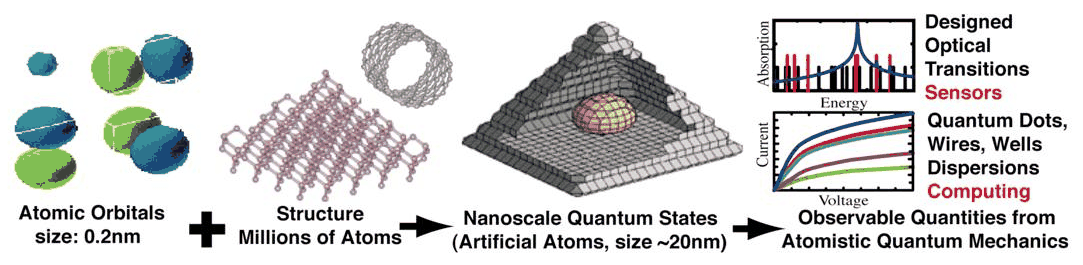
Slide 4: from atomic orbitals to observables — Slide 4 (top): atomic orbitals of about 0.2 nm combined over a structure of millions of atoms give the quantum states of an artificial atom of about 20 nm, from which observables such as optical transitions and currents follow.

How large is "millions of atoms"? Zincblende has 8 atoms in a cubic cell of side $a$, so the atom density is $8/a^3$. With 20 orbitals per atom (sp3d5s* with spin, lecture 21.3) the Hamiltonian has $20N$ rows for $N$ atoms.

Code10 lines · cell 3

P = nemo.structures.materials.load("klimeck2002_sp3s")
GAAS, INAS = P["GaAs"], P["InAs"]
a = GAAS.lattice_constant
density = 8 / a**3                                   # atoms per nm^3
print(f"GaAs: a = {a:.5f} nm, {density:.1f} atoms/nm^3")
for side in (11.3, 33.9, 101.7):
    n_at = density * side**3
    print(f"cube of {side:6.1f} nm: {n_at / 1e6:7.2f} million atoms, "
          f"{20 * n_at:.2e} rows of the sp3d5s* + spin Hamiltonian")
print(f"52 million atoms of GaAs fill a cube of {(52e6 / density)**(1 / 3):.1f} nm")

GaAs: a = 0.56660 nm, 44.0 atoms/nm^3
cube of   11.3 nm:    0.06 million atoms, 1.27e+06 rows of the sp3d5s* + spin Hamiltonian
cube of   33.9 nm:    1.71 million atoms, 3.43e+07 rows of the sp3d5s* + spin Hamiltonian
cube of  101.7 nm:   46.26 million atoms, 9.25e+08 rows of the sp3d5s* + spin Hamiltonian
52 million atoms of GaAs fill a cube of 105.7 nm

A cube of 101.7 nm of GaAs holds 46.3 million atoms; 52 million atoms of GaAs would fill a cube of 105.7 nm, so the "(101 nm)³" of the slide is the same size up to the exact box shape and its material content. Either way the Hamiltonian has about $10^9$ rows: no dense method can touch it, and lecture 21.4 explains how NEMO 3-D finds its eigenstates.

2. The multi-scale chain#

Slide 6: the NEMO 3-D flow. Atom positions (about 10–50 million atoms) are constructed and relaxed; strain gives a piezoelectric potential; the valence electrons (0.5–10 million atoms) are described by sp3d5s\ tight binding with spin–orbit coupling, with external electric or magnetic fields, and the single-particle states give optical and electronic properties; electron–electron interactions among a few states are added self-consistently (Poisson + LDA) or with Slater determinants. Right: an InAs dot (red) in an InGaAs alloy, the bimodal bond lengths of InGaAs, an emission wavelength against composition compared with experiment, and Coulomb diamonds of a single impurity.*

The chain is sequential, each step feeding the next:

Geometry construction. The dot's shape, size and composition are guessed from what the experimentalists report or from micrographs (height, width, alloy concentrations around it).
Atomistic relaxation. A valence force field (lecture 21.2) moves every atom to minimize the elastic energy; the strain is a result, not an input. The relaxation domain is large (10–50 million atoms), because strain is long-ranged.
Strain and piezoelectric potential. The local strain follows from the relaxed bonds, and from it the piezoelectric polarization and its potential, which enter the Hamiltonian as a perturbation.
Hamiltonian construction. The relaxed positions are frozen; every atom contributes its orbitals, with couplings that depend on the bond lengths and directions (lecture 21.3). The electronic domain can be smaller than the mechanical one (0.5–10 million atoms).
Single-particle states. A few eigenstates in the gap region are computed (lecture 21.4) and give optical transitions or transport properties.
Many-body interactions for a few electrons: self-consistent potentials, or Slater determinants for genuine electron–electron interaction (e.g. the Coulomb diamonds of single phosphorus or arsenic impurities in silicon, discussed later in the course).

The cells below run steps 1–5 on a small InAs pyramid (base 9 nm, height 3.5 nm, on a one-monolayer wetting layer) in a GaAs box of 18 × 18 × 10 cubic cells (10.2 × 10.2 × 5.7 nm), periodic in all directions. To keep the run short the electronic model is sp3s* (5 orbitals per atom without spin) from the NEMO 3-D paper (Klimeck et al. 2002); the full sp3d5s* with spin has 20.

Code22 lines · cell 5

timing = {}
t0 = time.perf_counter()
lat = nemo.structures.lattice.from_material(GAAS)
NXY, NZ, BASE, HEIGHT = 18, 10, 9.0, 3.5
cell, basis, sub = lat.conventional, lat.conventional_basis, lat.conventional_sublattice
g = np.stack(np.meshgrid(np.arange(NXY), np.arange(NXY), np.arange(NZ), indexing="ij"), -1).reshape(-1, 3)
X = ((g @ cell)[:, None, :] + basis[None]).reshape(-1, 3)
sublat = np.tile(sub, len(g))
species = [lat.species[i] for i in sublat]
c0 = np.array([NXY * a / 2, NXY * a / 2, 1.5])                  # centre of the pyramid base
zr = X[:, 2] - c0[2]
half = BASE / 2 * (1 - zr / HEIGHT)
in_pyr = (zr >= 0) & (zr <= HEIGHT) & (np.abs(X[:, 0] - c0[0]) <= half) & (np.abs(X[:, 1] - c0[1]) <= half)
wet = (zr >= -a / 4 - 1e-9) & (zr < 0)
for i in np.flatnonzero(in_pyr | wet):
    if species[i] == "Ga":
        species[i] = "In"
periods = np.diag([NXY * a, NXY * a, NZ * a])
ideal = Structure(X, species, periods, sublat, lat)
timing["1 geometry"] = time.perf_counter() - t0
print(f"{ideal.num_atoms} atoms, {species.count('In')} In, {species.count('Ga')} Ga, "
      f"{species.count('As')} As")

25920 atoms, 2220 In, 10740 Ga, 12960 As

Code23 lines · cell 6

# Martin's Keating constants (alpha, beta in N/m), with the ideal bond lengths of the electronic model
KEATING = {("Ga", "As"): (41.19, 8.95, np.sqrt(3) / 4 * a),
           ("In", "As"): (35.18, 5.50, np.sqrt(3) / 4 * INAS.lattice_constant)}
t0 = time.perf_counter()
relaxed = M.relax(M.Keating(ideal, parameters=KEATING), tol=1e-6)
timing["2 relaxation (Keating)"] = time.perf_counter() - t0
moved = np.linalg.norm(relaxed["positions"] - X, axis=1)
print(f"L-BFGS iterations {relaxed['iterations']}, largest force left {relaxed['max_force']:.1e} eV/nm, "
      f"largest displacement {moved.max():.3f} nm")

t0 = time.perf_counter()
strain = M.atomic_strain(ideal, relaxed["positions"],
                         lattice_constants={("In", "As"): INAS.lattice_constant, ("Ga", "As"): a})
timing["3 strain"] = time.perf_counter() - t0
sp = np.array(species)
tr = strain["hydrostatic"]
inner = strain["valid"] & (sp == "In") & in_pyr
outer = strain["valid"] & (sp == "Ga")
print(f"tr(eps) on In atoms of the pyramid: mean {100 * tr[inner].mean():.2f} %  "
      f"(InAs squeezed toward the GaAs lattice: (a_GaAs - a_InAs)/a_InAs = "
      f"{100 * (a - INAS.lattice_constant) / INAS.lattice_constant:.2f} % per axis)")
print(f"tr(eps) on Ga atoms of the barrier: mean {100 * tr[outer].mean():.3f} %, "
      f"range {100 * tr[outer].min():.2f} to {100 * tr[outer].max():.2f} %")

L-BFGS iterations 235, largest force left 8.7e-07 eV/nm, largest displacement 0.102 nm
tr(eps) on In atoms of the pyramid: mean -9.31 %  (InAs squeezed toward the GaAs lattice: (a_GaAs - a_InAs)/a_InAs = -6.48 % per axis)
tr(eps) on Ga atoms of the barrier: mean -2.224 %, range -4.47 to -0.77 %

Code20 lines · cell 7

t0 = time.perf_counter()
dotmat = nemo.structures.materials.alloy(GAAS, INAS)
relaxed_s = Structure(relaxed["positions"], species, periods, sublat, lat)
sk = nemo.models.tb.SlaterKoster(dotmat, spin=False, strain="bond_length", bond_tolerance=0.15)
H = sk.build(relaxed_s).at(np.zeros(3))
timing["4 Hamiltonian"] = time.perf_counter() - t0
print(f"H: {H.shape[0]} rows ({H.shape[0] // ideal.num_atoms} orbitals per atom), {H.nnz} non-zeros "
      f"({H.nnz / H.shape[0]:.0f} per row), {H.nnz / H.shape[0]**2:.1e} filled")

t0 = time.perf_counter()
res = lanczos_window_eigenstates(H, (0.5, 1.6), tol=1e-8, count=3)
timing["5 eigenstates (Lanczos)"] = time.perf_counter() - t0
norb = H.shape[0] // ideal.num_atoms
on_in = np.repeat(sp == "In", norb)
for e, v in zip(res["energies"], res["vectors"].T):
    p = np.abs(v)**2
    print(f"electron level {e:.4f} eV, weight on In atoms {p[on_in].sum() / p.sum():.2f}")
e_gaas = np.linalg.eigvalsh(nemo.models.tb.SlaterKoster(GAAS).build(bulk(lat)).dense(np.zeros(3)))
print(f"{res.attrs['steps']} Lanczos steps; bulk GaAs conduction-band edge of this model: "
      f"{e_gaas[e_gaas > 0.5].min():.4f} eV")

H: 129600 rows (5 orbitals per atom), 2410560 non-zeros (19 per row), 1.4e-04 filled
electron level 1.2775 eV, weight on In atoms 0.30
electron level 1.4494 eV, weight on In atoms 0.31
electron level 1.4593 eV, weight on In atoms 0.24
1600 Lanczos steps; bulk GaAs conduction-band edge of this model: 1.4173 eV

Code13 lines · cell 8

total = sum(timing.values())
for k, v in timing.items():
    print(f"{k:26s} {v:6.2f} s  ({100 * v / total:4.1f} %)")
print(f"{'total':26s} {total:6.2f} s")

fig, (a1, a2) = plt.subplots(1, 2, figsize=(11, 4))
sel = strain["valid"] & (np.abs(X[:, 1] - c0[1]) < a / 4)          # one (010) slice through the dot
sc = a1.scatter(X[sel, 0], X[sel, 2], c=100 * tr[sel], s=10, cmap=style.SIGNED, vmin=-10, vmax=10)
fig.colorbar(sc, ax=a1, label="tr ε (%)")
a1.set(xlabel="x (nm)", ylabel="z (nm)", title="tr ε on a (010) slice through the dot", aspect="equal")
a2.barh(list(timing)[::-1], list(timing.values())[::-1], color=style.OPEN_NEMO)
a2.set(xlabel="wall time (s)", title=f"{ideal.num_atoms} atoms, sp3s*, 2 threads")
fig.tight_layout()

1 geometry                   0.00 s  ( 0.0 %)
2 relaxation (Keating)       1.26 s  (16.2 %)
3 strain                     0.24 s  ( 3.0 %)
4 Hamiltonian                1.25 s  (16.0 %)
5 eigenstates (Lanczos)      5.06 s  (64.8 %)
total                        7.80 s

Figure computed by the notebook with open-nemo

The chain behaves as the lecture describes. The InAs is compressed by about 9 % in volume (the trace of the strain tensor, $\mathrm{tr}\,\varepsilon = \varepsilon_{xx}+\varepsilon_{yy}+ \varepsilon_{zz}$, measured from the InAs lattice: −9.31 % on average over the pyramid's In atoms). The GaAs around it is strained too, with $\mathrm{tr}\,\varepsilon$ between −0.77 % and −4.47 %: in this small periodic box the dot and its wetting layer press on the barrier everywhere. Strain is long-ranged, which is why NEMO 3-D's mechanical domain is larger than its electronic one. The Hamiltonian is extremely sparse: each row couples an orbital only to the orbitals of its own atom and its four neighbours. The pyramid binds one electron level, at 1.2775 eV, 140 meV below the GaAs conduction band edge (1.4173 eV), with 30 % of its weight on the In atoms; the next two levels found, at 1.4494 and 1.4593 eV, lie above the band edge: they are states of the GaAs in the finite box, not bound to the dot.

The eigenvalue step dominates the time, followed by the Hamiltonian and the relaxation. In NEMO 3-D each step was parallelized, and all of them scale linearly with the number of atoms: the relaxation and the Hamiltonian because each atom has four neighbours, the Lanczos solver because it only needs products of $H$ with vectors, whose cost is proportional to the number of non-zeros.

Slide 4: end-to-end wall time — Slide 4 (bottom): end-to-end NEMO 3-D wall time against system size on 8 to 128 cores; 52 million atoms took about 33 hours on 128 cores, on a straight line.

A rough check of that number: the time per non-zero of one product $H\mathbf{v}$, measured here, times the non-zeros of the 52-million-atom sp3d5s* + spin Hamiltonian (20 rows per atom, each coupled to 20 orbitals on 5 atoms), times the number of products of a Lanczos run with its second pass for the eigenvectors (here about 2 × 1000; NEMO 3-D ran 1000–5000 steps), divided by 128 cores.

Code10 lines · cell 10

v = np.random.default_rng(0).standard_normal(H.shape[0]) + 0j
t0 = time.perf_counter()
for _ in range(20):
    w = H @ v
t_nnz = (time.perf_counter() - t0) / 20 / H.nnz
nnz_52m = 52e6 * 20 * 5 * 20
for steps in (1000, 5000):
    hours = t_nnz * nnz_52m * 2 * steps / 128 / 3600
    print(f"{1e9 * t_nnz:.2f} ns per non-zero here; {steps} steps x 2 passes, 52 M atoms on 128 cores: "
          f"{hours:.1f} h of products")

0.60 ns per non-zero here; 1000 steps x 2 passes, 52 M atoms on 128 cores: 0.3 h of products
0.60 ns per non-zero here; 5000 steps x 2 passes, 52 M atoms on 128 cores: 1.4 h of products

On today's cores the products alone would take 0.3 to 1.3 hours on 128 cores, 25 to 100 times less than the 33 hours measured around 2007. The estimate leaves out the communication between the cores, the relaxation of a mechanical domain larger than the electronic one, the Hamiltonian construction and the storage of eigenvectors, and a core of 2007 was several times slower than the one used here. It is not a reconstruction of the old run; what it shows is the lecture's point that the cost is a fixed amount of work per non-zero, so nothing in the chain grows faster than the number of atoms.

3. InGaAs: bimodal bonds, not a virtual crystal#

In a macroscopic picture, In$x$Ga${1-x}$As is an alloy with an average lattice constant that interpolates linearly between GaAs and InAs (Vegard's law), and every cation–anion bond would have the length $\sqrt{3}\,a(x)/4$. Atomistically this is wrong: the In–As bonds stay close to the InAs bond length and the Ga–As bonds close to the GaAs one; every In pushes its As neighbours away and every Ga pulls them in. The distribution of bond lengths is bimodal, and the alloy is not a crystal in the strict sense. The valence-force-field relaxation produces this without any extra input.

Below, periodic supercells of 6 × 6 × 6 cubic cells (1728 atoms) with the cations drawn at random are relaxed with Keating's force field, letting the period "breathe" (NEMO 3-D's periodic boundary condition) so that each composition finds its own lattice constant.

Code35 lines · cell 12

def bond_lengths(s, positions, box):
    # cation-anion bond lengths and the cation species of each bond, in a periodic box
    wrapped = np.mod(positions, box)
    wrapped[wrapped >= box] = 0.0
    pairs = cKDTree(wrapped, boxsize=box).query_pairs(0.29, output_type="ndarray")
    d = positions[pairs[:, 1]] - positions[pairs[:, 0]]
    d = np.linalg.norm((d + box / 2) % box - box / 2, axis=1)
    spc = np.array(s.species)
    cation = np.where(spc[pairs[:, 0]] == "As", spc[pairs[:, 1]], spc[pairs[:, 0]])
    return d, cation


base = supercell(lat, 6)
xs = np.linspace(0, 1, 9)
stats, a_alloy, hist = {"In": [], "Ga": []}, [], {}
t0 = time.perf_counter()
for x in xs:
    s = random_alloy(base, "Ga", "In", x, seed=1)
    r = M.relax(M.Keating(s, parameters=KEATING), tol=1e-6, cell=True)
    box = np.diag(np.asarray(r["periods"]))
    d, cat = bond_lengths(s, r["positions"], box)
    a_alloy.append(box.mean() / 6)
    for c in stats:
        stats[c].append((d[cat == c].mean(), d[cat == c].std()) if (cat == c).any() else (np.nan, np.nan))
    if abs(x - 0.5) < 1e-9:
        hist = {c: d[cat == c] for c in stats}
stats = {c: np.array(v) for c, v in stats.items()}
a_alloy = np.array(a_alloy)
print(f"9 compositions relaxed in {time.perf_counter() - t0:.1f} s")
print(f"{'x':>5s} {'a (nm)':>8s} {'Vegard a':>9s} {'In-As (nm)':>11s} {'Ga-As (nm)':>11s} "
      f"{'Vegard bond':>12s}")
a_veg = (1 - xs) * a + xs * INAS.lattice_constant
for i, x in enumerate(xs):
    print(f"{x:5.3f} {a_alloy[i]:8.4f} {a_veg[i]:9.4f} {stats['In'][i, 0]:11.4f} {stats['Ga'][i, 0]:11.4f} "
          f"{np.sqrt(3) * a_veg[i] / 4:12.4f}")

9 compositions relaxed in 2.0 s
    x   a (nm)  Vegard a  In-As (nm)  Ga-As (nm)  Vegard bond
0.000   0.5666    0.5666         nan      0.2453       0.2453
0.125   0.5710    0.5715      0.2577      0.2458       0.2475
0.250   0.5755    0.5764      0.2584      0.2463       0.2496
0.375   0.5802    0.5813      0.2592      0.2468       0.2517
0.500   0.5850    0.5862      0.2598      0.2473       0.2538
0.625   0.5900    0.5911      0.2604      0.2477       0.2560
0.750   0.5952    0.5960      0.2611      0.2481       0.2581
0.875   0.6004    0.6009      0.2617      0.2485       0.2602
1.000   0.6058    0.6058      0.2623         nan       0.2623

Code14 lines · cell 13

fig, (a1, a2) = plt.subplots(1, 2, figsize=(11, 4))
cols = {"In": style.OPEN_NEMO, "Ga": style.CONTEXT}
for c in ("In", "Ga"):
    a1.errorbar(xs, stats[c][:, 0], yerr=stats[c][:, 1], color=cols[c], marker="o", capsize=3,
                label=f"{c}–As bonds (mean ± σ)")
    a2.hist(hist[c], bins=30, color=cols[c], alpha=0.8, label=f"{c}–As")
a1.plot(xs, np.sqrt(3) * a_veg / 4, "k--", lw=1, label="Vegard: √3 a(x)/4")
a1.set(xlabel="In fraction x", ylabel="bond length (nm)",
       title="relaxed random InₓGa₁₋ₓAs (1728 atoms)")
a1.legend(frameon=False, fontsize=8)
a2.axvline(np.sqrt(3) * a_veg[4] / 4, color="k", ls="--", lw=1, label="Vegard bond")
a2.set(xlabel="bond length (nm)", ylabel="number of bonds", title="x = 0.5: a bimodal distribution")
a2.legend(frameon=False, fontsize=8)
fig.tight_layout()

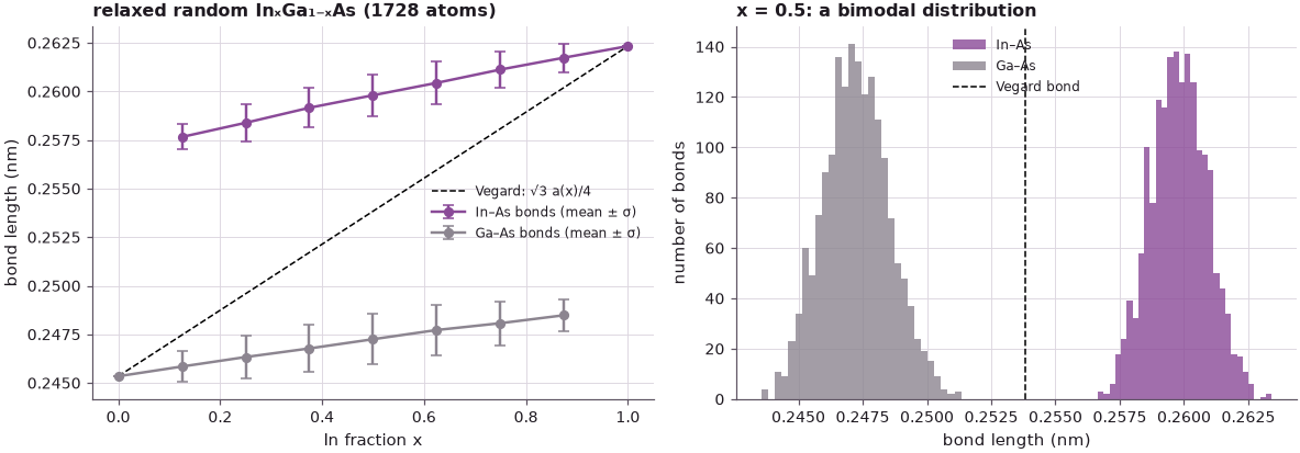
The lattice constant of the relaxed supercell follows Vegard's law closely (at most 0.0012 nm below it), yet no bond has the Vegard length: at $x = 0.5$ the In–As bonds average 0.2598 nm and the Ga–As bonds 0.2473 nm, against 0.2538 nm for the virtual crystal, and the two distributions do not overlap. From $x = 0.125$ to $0.875$ the In–As bond grows by 0.0040 nm and the Ga–As bond by 0.0027 nm, while the Vegard bond grows by 0.0127 nm: each bond follows the average by only a fifth to a third, in agreement with the EXAFS measurements of Mikkelsen and Boyce (1982) shown on slide 6. This local structure changes the electronic states (lecture 21.3) and is one reason NEMO 3-D represents alloys atom by atom; the benchmark notebook on the 2002 NEMO 3-D paper compares these bond lengths with the paper's Fig. 9.

Summary#

NEMO 3-D is atomistic because nanostructures have countable atoms, uses local orbitals because the structures are finite, and is empirical because semiconductor bonds are stable.
A $(101.7\ \mathrm{nm})^3$ GaAs cube holds 46.3 million atoms and gives an sp3d5s* + spin Hamiltonian of $9.25\times10^8$ rows.
The chain geometry → Keating relaxation → strain → strained tight-binding Hamiltonian → Lanczos runs here end to end on a 25,920-atom InAs pyramid in GaAs in about 8 s; it binds one electron level 140 meV below the GaAs band edge. The eigenvalue step takes about two thirds of the time, and every step scales linearly with the number of atoms.
Relaxed random InGaAs follows Vegard's law for the lattice constant but has bimodal bond lengths (0.2598 and 0.2473 nm at $x = 0.5$ against 0.2538 nm).

Exercises#

Make the pyramid larger (BASE = 11, HEIGHT = 4.5, with NXY = 20) and rerun section 2. How do the electron level and its weight on the In atoms change? How does each step's time scale with the number of atoms?
Double the bond-bending constant β of both materials in KEATING and rerun section 2. How do the hydrostatic strain in the dot and the electron level change?
In section 3, plot the standard deviation of the In–As bond lengths against $x$. Where is the disorder largest, and why?