Lecture 10.5

Introduction to transport — free charge interacting with the electrostatic potential: an NIN diode

In the lecture

the semiclassical electron density of a bulk semiconductor: the Fermi–Dirac integral $n = N_C\mathcal F_{1/2}(\eta_F)$ and its non-degenerate (Boltzmann) limit
the Fermi level of GaAs doped to $2\cdot10^{18}$ cm$^{-3}$ (about 80 meV above the band edge) and of nearly intrinsic GaAs at $10^{15}$ cm$^{-3}$ (about 160 meV below it)
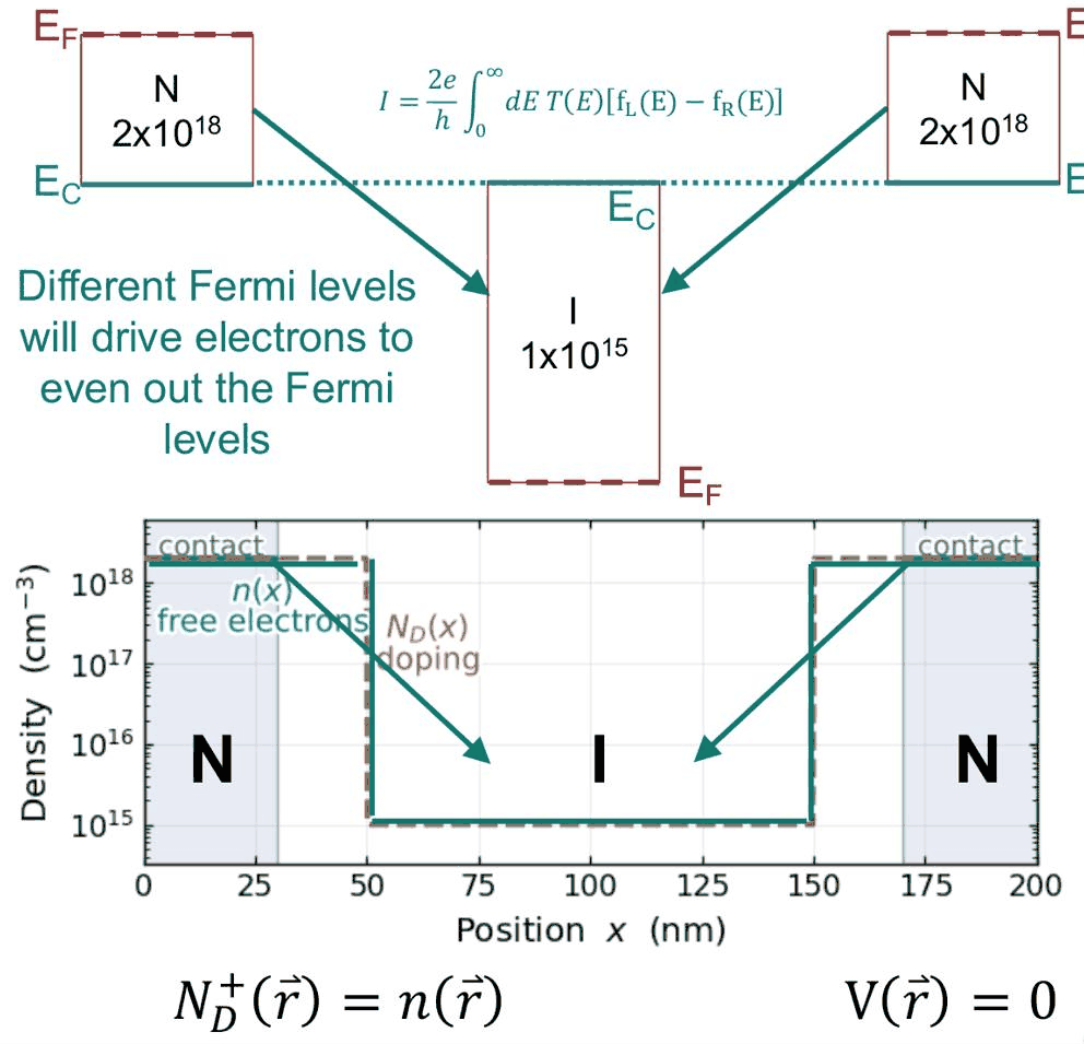
three adjacent layers, N–I–N: with flat bands the three Fermi levels do not line up, and electrons flow to even them out
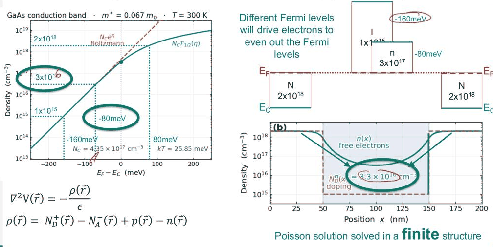
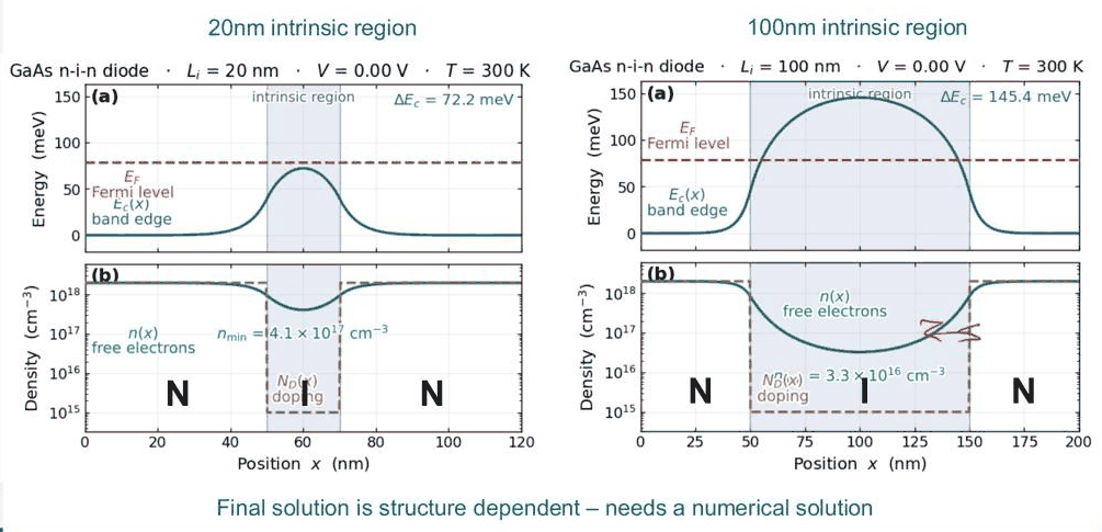
in equilibrium the Fermi level is flat; electrons diffuse into the intrinsic region, the charge imbalance bends the bands, and Poisson's equation sets the final profile
the profile depends on the structure (20 nm versus 100 nm intrinsic region) and needs a numerical solution; degenerate contacts need the full Fermi–Dirac integral

In this notebook

you compute the bulk density–Fermi level relation for GaAs with open-nemo's Fermi–Dirac integral, solve the NIN diode at equilibrium with nemo.semiclassical (Fermi–Dirac statistics and Poisson's equation), check charge neutrality and the depletion and accumulation charges, compare the 20 nm and 100 nm intrinsic regions, and show what Boltzmann statistics would get wrong.

Run the notebookEvery number and figure on this page comes from it. Change it, rerun it, take it further.

Download .ipynb View on GitHub

Run it on your own machine

The notebook needs open-nemo (Python ≥ 3.10 and a C++20 compiler; BLAS/LAPACK).

git clone https://github.com/denphi/open-nemo.git && cd open-nemo
python3 -m venv .venv && source .venv/bin/activate
pip install -e ".[notebooks]"
jupyter lab From_Atoms_to_Devices/05_introduction_to_transport/10_5_nin_diode.ipynb

Code10 lines · cell 1

import numpy as np
import matplotlib.pyplot as plt
from scipy.optimize import brentq
import opennemo as nemo
from opennemo.visualization import style
from opennemo.structures.statistics import fermi_dirac_half

style.use(notebook=True)
EM = nemo.structures.materials.EffectiveMassMaterial
KB, M0_HBAR2 = nemo.core.units.KB, nemo.core.units.M0_HBAR2      # eV/K; m0/ħ² in 1/(eV nm²)

1. The semiclassical electron density#

So far the potential was given: flat, or with a voltage drop assumed by hand. Now the electrons themselves enter. In a bulk semiconductor with a parabolic conduction band of effective mass $m^*$, the electron density for a Fermi level $E_F$ is

n = N_C\,\mathcal F_{1/2}(\eta_F),\qquad \eta_F = \frac{E_F - E_C}{k_BT},\qquad \mathcal F_{1/2}(\eta) = \frac{2}{\sqrt\pi}\int_0^\infty\frac{\sqrt\epsilon\,d\epsilon}{1 + e^{\epsilon - \eta}}, \qquad N_C = 2\left(\frac{2\pi m^*k_BT}{h^2}\right)^{3/2},

with $E_C$ the conduction-band edge, $k_BT$ the thermal energy and $N_C$ the effective density of states. For a Fermi level well below the band edge (low doping, non-degenerate) the Fermi function becomes a Boltzmann factor and $n \approx N_C e^{\eta_F}$. Klimeck calls the Fermi–Dirac result the ground truth at the semiclassical level; the two agree at low density and separate once the Fermi level approaches the band edge. fermi_dirac_half in opennemo.structures.statistics is the normalized $\mathcal F_{1/2}$ above.

Code29 lines · cell 3

T = 300.0
kt = KB * T
m_eff = 0.067
Nc = 2 * (m_eff * M0_HBAR2 * kt / (2 * np.pi)) ** 1.5 * 1e21          # nm⁻³ -> cm⁻³
print(f"k_B T = {kt * 1e3:.2f} meV, N_C = {Nc:.3e} cm⁻³")


def fermi_level(n):
    # E_F - E_C (eV) with n = N_C F_1/2((E_F - E_C)/kT)
    return brentq(lambda e: Nc * fermi_dirac_half(e / kt) - n, -1.0, 1.0)


for n in (2e18, 1e15):
    print(f"n = {n:.0e} cm⁻³: E_F - E_C = {fermi_level(n) * 1e3:7.2f} meV (Fermi-Dirac),"
          f" {kt * np.log(n / Nc) * 1e3:7.2f} meV (Boltzmann)")

gaas = EM("GaAs", m_eff, 12.9)
bulk = nemo.Heterostructure1D([nemo.Layer(gaas, 20, donors=2e18)], spacing=0.25)
print(f"open-nemo contact Fermi level for 2e18 cm⁻³: {bulk.contact_fermi_level('left', T) * 1e3:.2f} meV")

eta = np.linspace(-250, 250, 501) * 1e-3 / kt
fig, ax = plt.subplots(figsize=(6.5, 4))
ax.semilogy(eta * kt * 1e3, Nc * fermi_dirac_half(eta), color=style.OPEN_NEMO, label="N_C F_1/2(η)")
ax.semilogy(eta * kt * 1e3, Nc * np.exp(eta), "--", color=style.CONTEXT, label="N_C e^η (Boltzmann)")
for n in (2e18, 1e15):
    ax.plot(fermi_level(n) * 1e3, n, "o", color=style.REFERENCE, ms=5)
ax.set(xlabel="E_F − E_C (meV)", ylabel="electron density (cm⁻³)", ylim=(1e13, 1e19),
       title="GaAs conduction band, m* = 0.067 m₀, 300 K")
ax.legend(frameon=False, fontsize=8);

k_B T = 25.85 meV, N_C = 4.352e+17 cm⁻³
n = 2e+18 cm⁻³: E_F - E_C =   79.06 meV (Fermi-Dirac),   39.43 meV (Boltzmann)
n = 1e+15 cm⁻³: E_F - E_C = -157.05 meV (Fermi-Dirac), -157.07 meV (Boltzmann)
open-nemo contact Fermi level for 2e18 cm⁻³: 79.04 meV

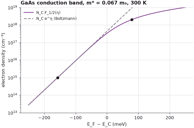
Figure computed by the notebook with open-nemo

The numbers match the lecture's plot: $N_C = 4.35\cdot10^{17}$ cm$^{-3}$ and $k_BT = 25.85$ meV. A doping of $2\cdot10^{18}$ cm$^{-3}$ needs the Fermi level 79.06 meV above the band edge ("ballpark 80 meV"), and open-nemo's contact Fermi level agrees (79.04 meV). Boltzmann statistics would put it at only 39.43 meV: for degenerate doping the non-degenerate formula is far off. For $10^{15}$ cm$^{-3}$ both give $-157$ meV, the lecture's $-160$ meV.

2. Three adjacent materials: what should the band alignment be?#

Now put three GaAs layers next to each other: N ($2\cdot10^{18}$ cm$^{-3}$, 50 nm), I (nominally undoped, $10^{15}$ cm$^{-3}$, 100 nm), N ($2\cdot10^{18}$ cm$^{-3}$, 50 nm). Since all three are GaAs, the first guess is a flat conduction band, zero field everywhere and each layer neutral ($N_D^+ = n$, $V = 0$). But then the Fermi level is 79 meV above the band edge in the contacts and 157 meV below it in the middle. Different Fermi levels drive electrons from the contacts into the intrinsic region to even them out.

Slide 6: flat bands leave the Fermi levels out of line — Slide 6: with a flat conduction band the three layers have different Fermi levels; the density follows the doping exactly.

3. In equilibrium the Fermi level is flat#

In equilibrium there is one Fermi level, flat through the whole device, by definition. Klimeck calls this one of the key recipes for sketching any real device: start with the Fermi level, then draw the band edges. The electrons that diffuse into the intrinsic region leave the ionized donors behind; the resulting charge bends the bands, and the electrostatic potential must satisfy Poisson's equation,

\frac{d}{dx}\Bigl(\epsilon\frac{d\phi}{dx}\Bigr) = -e\bigl[N_D^+(x) - n(x)\bigr],\qquad n(x) = N_C\,\mathcal F_{1/2}\!\left(\frac{E_F - E_C(x)}{k_BT}\right),\qquad E_C(x) = E_C^0 - e\phi(x).

nemo.semiclassical solves this nonlinear problem (Thomas–Fermi electrostatics with Fermi–Dirac statistics) on the 1-D device, with the Fermi level of the contacts and no field at the boundaries.

Code26 lines · cell 5

def nin(intrinsic, contact=50.0, dx=0.25):
    layers = [nemo.Layer(gaas, contact, donors=2e18), nemo.Layer(gaas, intrinsic, donors=1e15),
              nemo.Layer(gaas, contact, donors=2e18)]
    return nemo.Heterostructure1D(layers, spacing=dx)


dev = nin(100.0)
mu = dev.contact_fermi_level("left", T)
sol = nemo.semiclassical(dev, mu, temperature=T)
x, ec, n = dev.x, sol["band_edge"], sol["electron_density"]
mid = np.argmin(abs(x - x[-1] / 2))
print(f"Fermi level {mu * 1e3:.2f} meV above the contact band edge")
print(f"band-edge rise in the centre: {(ec[mid] - ec[0]) * 1e3:.1f} meV")
print(f"centre: n = {n[mid]:.3g} cm⁻³, E_F - E_C = {(mu - ec[mid]) * 1e3:.1f} meV;"
      f" bulk relation for this n: {fermi_level(n[mid]) * 1e3:.1f} meV")

fig, axes = plt.subplots(2, 1, figsize=(7.5, 6), sharex=True)
axes[0].plot(x, ec * 1e3, color=style.OPEN_NEMO, label="E_C(x)")
axes[0].axhline(mu * 1e3, color=style.REFERENCE, ls="--", lw=1, label="E_F (flat)")
axes[0].set(ylabel="energy (meV)", title="NIN diode at equilibrium, 50 | 100 | 50 nm")
axes[0].legend(frameon=False, fontsize=8)
axes[1].semilogy(x, n, color=style.OPEN_NEMO, label="n(x), free electrons")
axes[1].semilogy(x, dev.donors, "--", color=style.CONTEXT, label="N_D(x), doping")
axes[1].set(xlabel="position x (nm)", ylabel="density (cm⁻³)", ylim=(5e14, 5e18))
axes[1].legend(frameon=False, fontsize=8)
fig.tight_layout()

Fermi level 79.04 meV above the contact band edge
band-edge rise in the centre: 145.9 meV
centre: n = 3.2e+16 cm⁻³, E_F - E_C = -66.8 meV; bulk relation for this n: -66.8 meV

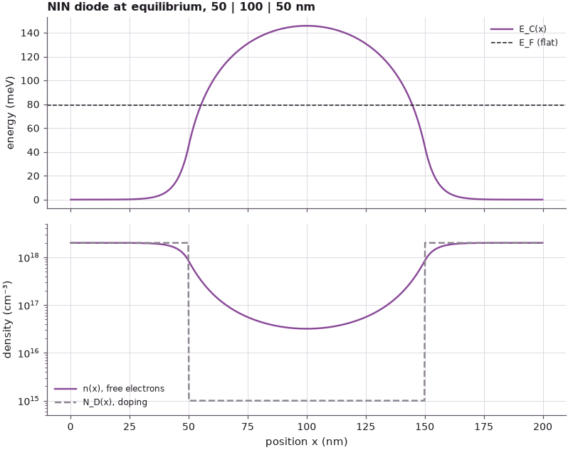
The conduction band rises by 145.9 meV in the middle of the intrinsic region, where the density falls to $3.2\cdot10^{16}$ cm$^{-3}$, much more than the doping of $10^{15}$ cm$^{-3}$ but far below the contacts. There the Fermi level is 66.8 meV below the band edge, not 157 meV: the intrinsic layer is flooded by electrons from the contacts. The lecture's solution (slide 8) shows the same profile, a band-edge rise of 145.4 meV and $3.3\cdot10^{16}$ cm$^{-3}$ in the centre (labelled "$3\times10^{17}$" on the slide, a typo Klimeck points out); his reading of $-80$ meV from the density plot is close to the computed $-66.8$ meV.

Slide 8: the equilibrium solution — Slide 8: the Poisson solution with a flat Fermi level; electrons spill into the intrinsic region and the band bends up.

4. Carriers diffuse to even out concentration differences#

The same result can be told as a drift–diffusion story: electrons diffuse from the heavily doped contacts into the intrinsic region to reduce the concentration gradient; the charge they carry builds up a field that drives them back. In equilibrium all processes and their reverse are present (drift balances diffusion) and no net current flows. The electrons that "don't belong" in the intrinsic region form a negative charge; the contacts near the junctions are depleted and carry the positive charge of the uncompensated donors. The whole device stays neutral.

Code10 lines · cell 7

rho = dev.donors - n                                         # net positive charge density / e (cm⁻³)
half = x < x[-1] / 2
to_cm2 = 1e-7                                                # cm⁻³ · nm -> cm⁻²
depleted = np.trapezoid(np.clip(rho[half], 0, None), x[half]) * to_cm2
accumulated = np.trapezoid(np.clip(-rho[half], 0, None), x[half]) * to_cm2
print(f"left half: depletion charge {depleted:.3e} cm⁻², electrons in excess {accumulated:.3e} cm⁻²")
print(f"net charge of the whole device: {np.trapezoid(rho, x) * to_cm2:.1e} cm⁻²"
      f" (doping integral {np.trapezoid(dev.donors, x) * to_cm2:.2e} cm⁻²)")
field = -np.gradient(sol["potential"], x)                    # V/nm
print(f"largest electric field: {abs(field).max() * 1e4:.0f} kV/cm")

left half: depletion charge 6.313e+11 cm⁻², electrons in excess 6.310e+11 cm⁻²
net charge of the whole device: -1.8e+07 cm⁻² (doping integral 2.00e+13 cm⁻²)
largest electric field: 87 kV/cm

Each junction transfers $6.3\cdot10^{11}$ electrons per cm$^2$ from the contact into the intrinsic region; the net charge of the device vanishes to one part in $10^{6}$ of the doping. The field that balances the diffusion reaches 87 kV/cm at the junctions.

5. The structure determines the potential profile#

How much the band bends depends on the structure. In a short intrinsic region the electrons from the two contacts overlap and keep the band low; in a long one the centre approaches the bulk intrinsic Fermi level.

Slide 11: 20 nm against 100 nm intrinsic region — Slide 11: equilibrium band edge and density for a 20 nm and a 100 nm intrinsic region.

Below the intrinsic length is varied from 5 nm to 400 nm, and for the 100 nm device the calculation is repeated with Boltzmann statistics (with the Boltzmann contact Fermi level), to show lesson 4 of the lecture.

Code26 lines · cell 9

print(" L_I (nm)   band-edge rise (meV)   n in the centre (cm⁻³)")
fig, axes = plt.subplots(1, 2, figsize=(11, 4))
for L, c in zip((5, 10, 20, 50, 100, 200, 400), style.sweep(7)):
    d = nin(float(L))
    s = nemo.semiclassical(d, mu, temperature=T)
    m = np.argmin(abs(d.x - d.x[-1] / 2))
    print(f"   {L:4d}          {(s['band_edge'][m] - s['band_edge'][0]) * 1e3:6.1f}"
          f"               {s['electron_density'][m]:.3g}")
    if L in (20, 100, 400):
        axes[0].plot(d.x - d.x[-1] / 2, s["band_edge"] * 1e3, color=c, label=f"L_I = {L} nm")
axes[0].axhline(mu * 1e3, color=style.REFERENCE, ls="--", lw=1)
axes[0].axhline((mu - fermi_level(1e15)) * 1e3, color=style.CONTEXT, ls=":", lw=1)
axes[0].set(xlabel="position from the centre (nm)", ylabel="E_C (meV)", xlim=(-250, 250),
            title="equilibrium band edge")
axes[0].legend(frameon=False, fontsize=8, loc="center right")

mu_b = kt * np.log(2e18 / Nc)
s_b = nemo.semiclassical(dev, mu_b, temperature=T, statistics="boltzmann")
rise_b = (s_b["band_edge"][mid] - s_b["band_edge"][0]) * 1e3
print(f"\n100 nm, Boltzmann: contact E_F - E_C = {mu_b * 1e3:.1f} meV, band-edge rise {rise_b:.1f} meV,"
      f" centre n = {s_b['electron_density'][mid]:.3g} cm⁻³")
axes[1].plot(x, (mu - ec) * 1e3, color=style.OPEN_NEMO, label="Fermi-Dirac")
axes[1].plot(x, (mu_b - s_b["band_edge"]) * 1e3, "--", color=style.CONTEXT, label="Boltzmann")
axes[1].set(xlabel="position x (nm)", ylabel="E_F − E_C (meV)", title="100 nm, statistics")
axes[1].legend(frameon=False, fontsize=8)
fig.tight_layout()

 L_I (nm)   band-edge rise (meV)   n in the centre (cm⁻³)
      5            27.3               1.23e+18
     10            46.5               8.08e+17
     20            72.4               4.06e+17
     50           113.0               1.07e+17
    100           145.9               3.2e+16
    200           178.9               9.09e+15
    400           209.0               2.84e+15

100 nm, Boltzmann: contact E_F - E_C = 39.4 meV, band-edge rise 109.9 meV, centre n = 2.85e+16 cm⁻³

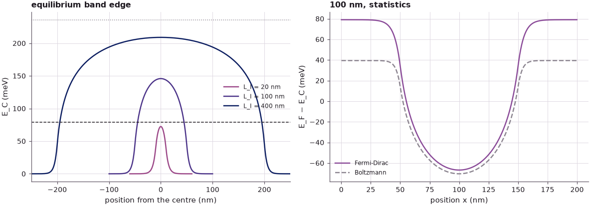
The 20 nm device has a band-edge rise of 72.4 meV and $4.06\cdot10^{17}$ cm$^{-3}$ in the centre (the lecture: 72.2 meV and $4.1\cdot10^{17}$ cm$^{-3}$); the 100 nm device 145.9 meV. The rise keeps growing with the length, 209.0 meV at 400 nm, toward the flat-band mismatch of $79 + 157 = 236$ meV that a very long intrinsic region would reach. The final solution is structure dependent and needs a numerical solution, as the slide says.

With Boltzmann statistics the contact Fermi level is 39.4 meV instead of 79.0 meV above the band edge, and the computed band-edge rise is 109.9 meV instead of 145.9 meV: a 25 % error in the barrier that any transport calculation would then see. Degenerate contacts need the full Fermi–Dirac integral.

Summary#

The semiclassical density is $n = N_C\mathcal F_{1/2}((E_F - E_C)/k_BT)$, with $N_C = 4.35\cdot10^{17}$ cm$^{-3}$ for GaAs at 300 K; $2\cdot10^{18}$ cm$^{-3}$ puts $E_F$ 79 meV above the band edge, $10^{15}$ cm$^{-3}$ 157 meV below it.
Doping variations cause potential variations even at equilibrium: in an NIN stack of a single material the band bends by 146 meV for a 100 nm intrinsic region.
In equilibrium the Fermi level is flat and the band edge bends; electrons diffuse into the intrinsic region ($6.3\cdot10^{11}$ cm$^{-2}$ per junction here) and the depleted contacts balance their charge.
Potential and free charge interact strongly; Poisson's equation ties them together, and the result depends on the structure (72 meV for 20 nm, 146 meV for 100 nm).
Degenerate contacts need Fermi–Dirac statistics: Boltzmann underestimates the barrier by 25 %.

Exercises#

Lower the contact doping to $10^{17}$ cm$^{-3}$ and repeat Sections 3 and 5. Does the Boltzmann error shrink, and why?
Replace the intrinsic layer by AlGaAs (EM("AlGaAs", 0.092, 12.2, conduction_band_edge=0.3)), which makes the NIN diode a single barrier. How much of the band-edge profile is band offset and how much electrostatics?
Compute the screening length of the contacts from the depletion profile of Section 4 and compare it with the Thomas–Fermi length $\sqrt{\epsilon\,k_BT\,\mathcal F_{1/2}(\eta)/(e^2 N_C\,\mathcal F_{-1/2}(\eta))}$ (use fermi_dirac_minus_half).