Lecture 13

Incoherent scattering concepts and impact in RTDs

In the lecture

where the valley current of an RTD comes from, and the question of the 1990s: is it scattering?
electron–phonon scattering in the resonator picture: a Fabry–Perot cavity with a vibrating mirror acquires sidebands, and the polar optical phonon produces an echo of the current peak in the valley
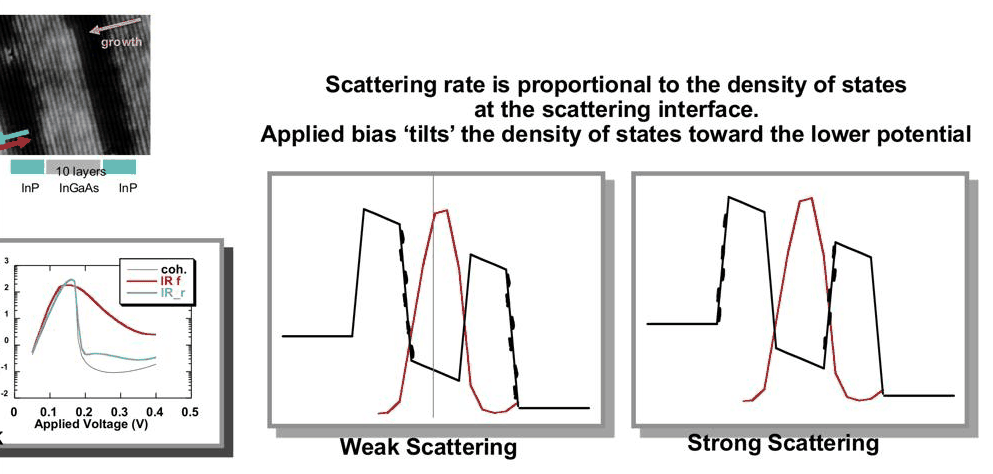
interface roughness scattering and why it makes the I–V asymmetric: bias leans the density of states against one interface
alloy disorder and transverse effective-mass effects: weak in GaAs/AlGaAs
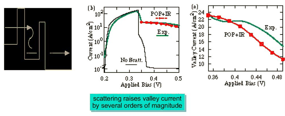
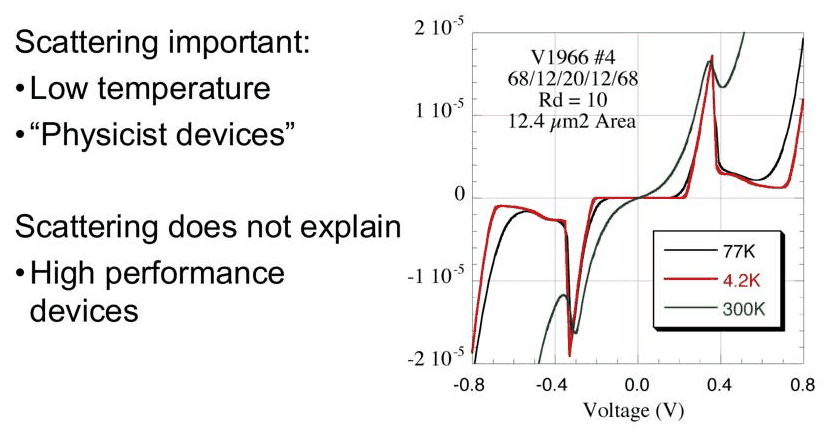
low temperature, where scattering raises the valley current by orders of magnitude, against room temperature, where scattering inside the RTD does not explain the valley current and the contacts and the band structure matter more

In this notebook

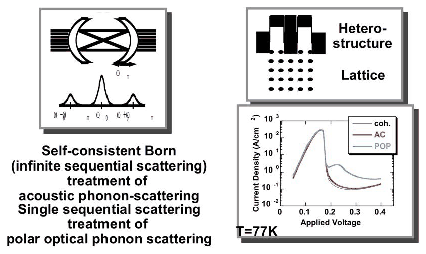
builds a GaAs/Al${0.3}$Ga${0.7}$As RTD on a monolayer grid, computes its Thomas–Fermi potential and then the current with NEMO's k-resolved scattering solver RoughnessTransport (Lake et al. 1997): coherent, with polar optical phonons, with interface roughness on one interface in forward and reverse bias, and with alloy disorder in the barriers, at 77 K and at 300 K; it shows the non-locality of the Fröhlich coupling, locates the phonon echo from the resonance trace, and varies the roughness correlation length.

Run the notebookEvery number and figure on this page comes from it. Change it, rerun it, take it further.

Download .ipynb View on GitHub

Run it on your own machine

The notebook needs open-nemo (Python ≥ 3.10 and a C++20 compiler; BLAS/LAPACK).

git clone https://github.com/denphi/open-nemo.git && cd open-nemo
python3 -m venv .venv && source .venv/bin/activate
pip install -e ".[notebooks]"
jupyter lab From_Atoms_to_Devices/06_resonant_tunneling_diodes/13_0_incoherent_scattering_in_rtds.ipynb

Code8 lines · cell 1

import numpy as np
import matplotlib.pyplot as plt
import opennemo as nemo
from opennemo.visualization import style

style.use(notebook=True)
H2M0 = nemo.core.units.HBAR2_2M0          # ħ²/2m₀ = 0.0381 eV nm²
EM = nemo.structures.materials.EffectiveMassMaterial

1. Where does the valley current come from?#

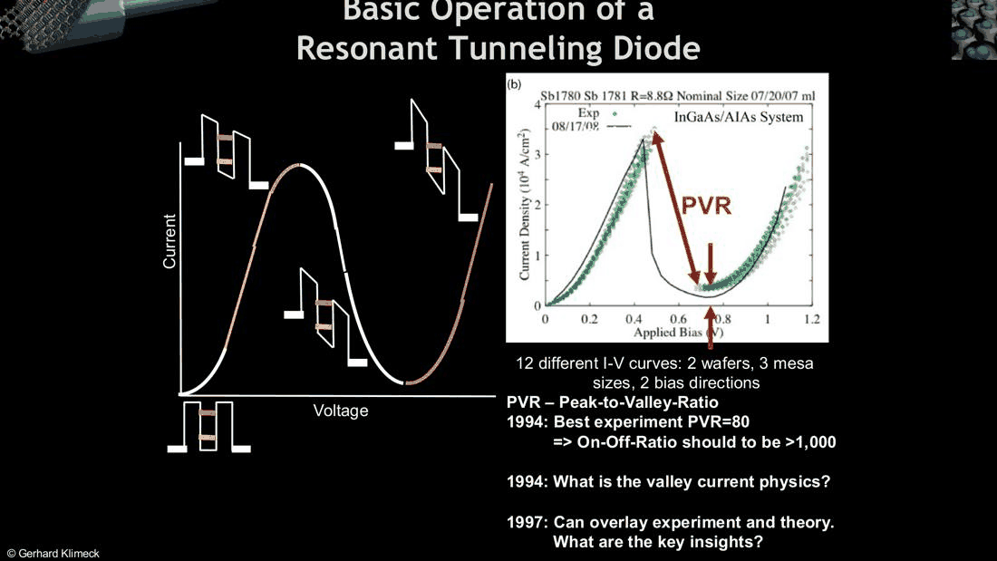
The figure of merit of an RTD for circuits is its peak-to-valley current ratio (PVR). Around 1994 the best measured PVR of an InGaAs/AlAs RTD was about 80, while circuit designers wanted on–off ratios above 1000, and simple coherent simulations predicted far larger ratios than measured. What carries the valley current? The usual first suspect is incoherent scattering: an electron that loses or gains energy inside the device, or changes its transverse momentum, can pass the double barrier even when the resonance is not aligned with the emitter. By 1997, NEMO simulations could be overlaid on measured I–V curves; this lecture summarises what the scattering models showed.

Slide 2: basic RTD operation and measured InGaAs/AlAs I–V curves with PVR — Slide 2. Band diagrams at different voltages and the resulting I–V; on the right, twelve measured I–V curves of an InGaAs/AlAs RTD (two wafers, three mesa sizes, two bias directions) overlaid with NEMO simulations. In 1994 the best experimental PVR was 80, the target above 1000.

2. The device and the coherent reference#

Scattering in NEMO is computed in the central (non-equilibrium) region: barriers and well. The model used here, opennemo.solvers.roughness.RoughnessTransport, follows Lake, Klimeck, Bowen and Jovanovic (J. Appl. Phys. 81, 7845 (1997)): the Green functions are resolved in the transverse wavevector $k$ (a radial grid of num_k points up to k_max), elastic scatterers (interface roughness, alloy disorder) are treated in the self-consistent Born approximation, and polar optical phonons in the single sequential approximation, with NEMO's reservoir relaxation (6.6 meV) in the contacts.

The device is a GaAs/Al${0.3}$Ga${0.7}$As RTD on a grid of one GaAs monolayer, $a = 0.2833$ nm: 20 nm contacts doped to $10^{18}$ cm$^{-3}$, 5 nm undoped spacers, 14-monolayer (4.0 nm) barriers and an 18-monolayer (5.1 nm) well. The potential is the Thomas–Fermi self-consistent one of lectures 11.2–11.3; the scattering is computed on that fixed potential.

Code57 lines · cell 5

from opennemo.solvers.roughness import (
    InterfaceRoughness,
    PolarOpticalPhonon,
    RoughnessTransport,
    ShortRangeScattering,
    energy_grid,
    froehlich_kernel,
)

ML, x_al, OFFSET = 0.2833, 0.3, 0.324
gaas = EM("GaAs", 0.067, 12.9, conduction_band_edge=0.0)
algaas = EM("Al0.3Ga0.7As", 0.067 + 0.083 * x_al, 12.9 - 2.84 * x_al, conduction_band_edge=OFFSET)
mixed = EM("rough monolayer", 0.067 + 0.083 * x_al / 2, 12.9 - 1.42 * x_al, conduction_band_edge=OFFSET / 2)


def make_rtd(rough=None):
    """RTD in monolayers; rough = 'emitter' or 'collector' puts a half-covered monolayer at that well interface."""
    well = {"emitter": [(mixed, 1, 0), (gaas, 17, 0)], "collector": [(gaas, 17, 0), (mixed, 1, 0)]}
    stack = (
        [(gaas, 70, 1e18), (gaas, 18, 0), (algaas, 14, 0)]
        + well.get(rough, [(gaas, 18, 0)])
        + [(algaas, 14, 0), (gaas, 18, 0), (gaas, 70, 1e18)]
    )
    return nemo.Heterostructure1D(
        [nemo.Layer(m, n * ML, donors=d) for m, n, d in stack],
        spacing=ML,
        mass_average="mean",
        terminal_layers=(2, 2),
    )


rtd = make_rtd()
V = np.round(np.arange(0.0, 0.5001, 0.025), 3)
T = 77
tf = nemo.thomas_fermi_iv(rtd, V, T)
MU = float(np.atleast_1d(tf["mu_left"])[0])
coh = RoughnessTransport(rtd, [], k_max=0.5, num_k=12)


def grid(tr, u, v, T):
    return energy_grid(tr, u, MU, MU - v, T, step=1e-3, current_only=True, resonances="on")


J_coh = np.array(
    [coh.solve(grid(coh, u, v, T), u, MU, MU - v, T)["current_density"] for v, u in zip(V, tf["potential"])]
)
k = int(np.argmax(J_coh))
kv = k + int(np.argmin(J_coh[k:]))
print(f"{rtd.num_sites} sites; emitter Fermi level {MU * 1e3:.1f} meV at {T} K")
print(
    f"coherent (k-resolved): peak {J_coh[k]:.0f} A/cm^2 at {V[k]:.3f} V, valley {J_coh[kv]:.0f} A/cm^2 at "
    f"{V[kv]:.3f} V, PVR {J_coh[k] / J_coh[kv]:.0f}"
)
print(
    f"thomas_fermi_iv current at the same biases: {tf['current_density'][k]:.0f} and "
    f"{tf['current_density'][kv]:.0f} A/cm^2"
)

222 sites; emitter Fermi level 53.7 meV at 77 K
coherent (k-resolved): peak 16064 A/cm^2 at 0.200 V, valley 423 A/cm^2 at 0.375 V, PVR 38
thomas_fermi_iv current at the same biases: 14931 and 381 A/cm^2

The two coherent currents differ by several per cent because they integrate over the transverse momentum differently: thomas_fermi_iv integrates analytically with the contact mass, RoughnessTransport sums a 12-point $k$ grid with the local mass of each layer (Lake's $V_k(z)$). All comparisons below are made within RoughnessTransport, with and without scattering, on the same grids.

3. Phonons: a resonator with a vibrating mirror#

The lecture's picture: an RTD is a Fabry–Perot resonator whose mirrors are the barriers. If a mirror vibrates at a discrete frequency $\omega$, light leaving the cavity acquires sidebands at $\pm\hbar\omega$. An electron in the well couples to the lattice vibrations in the same way. Acoustic phonons have a continuous, low-energy spectrum and mainly broaden the resonance; the polar optical (LO) phonon of GaAs has a nearly fixed energy $\hbar\omega_\text{LO} = 36$ meV, so an electron can enter the well by emitting one phonon when the resonance lies 36 meV below the emitter states. The result is a replica, an echo, of the current peak in the valley, displaced by one phonon energy, and visible at low temperature.

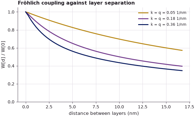
Slide 4: electron–phonon interaction as coupled resonators; acoustic and polar optical phonon I–V at 77 K — Slide 4. Electron–phonon interactions as coupled resonators (heterostructure and lattice). At 77 K, acoustic phonons in the self-consistent Born approximation (AC) and polar optical phonons in the single sequential approximation (POP) are compared with the coherent current (coh.): the POP current shows a shoulder in the valley.

The polar optical phonon couples through the long-range Coulomb field of the vibrating ions (the Fröhlich interaction), so its self-energy connects an electron on layer $L$ with layers $L + d$ far away. The weights $W[d]$ of froehlich_kernel show how slowly the coupling decays with distance; this non-locality is why the lecture states that the POP self-energy needs the full matrix, and that a tridiagonal approximation runs about ten times faster but misrepresents the strength.

Code17 lines · cell 9

kk = np.linspace(0, 0.5, 12)
W = froehlich_kernel(kk, 60, ML)
fig, ax = plt.subplots(figsize=(6.5, 3.6))
for j, c in zip((1, 4, 8), style.sweep(3)):
    ax.plot(np.arange(60) * ML, W[:, j, j] / W[0, j, j], color=c, lw=2, label=f"k = q = {kk[j]:.2f} 1/nm")
ax.set(
    xlabel="distance between layers (nm)",
    ylabel="W[d] / W[0]",
    ylim=(0, 1.05),
    title="Fröhlich coupling against layer separation",
)
ax.legend(fontsize=8)
for j in (1, 4, 8):
    print(
        f"k = q = {kk[j]:.2f} 1/nm: coupling at 5 nm is {W[int(round(5 / ML)), j, j] / W[0, j, j]:.2f} "
        "of the on-site value"
    )

k = q = 0.05 1/nm: coupling at 5 nm is 0.82 of the on-site value
k = q = 0.18 1/nm: coupling at 5 nm is 0.65 of the on-site value
k = q = 0.36 1/nm: coupling at 5 nm is 0.56 of the on-site value

Figure computed by the notebook with open-nemo

The polar optical phonon current at 77 K is computed with solve_phonon_current (GaAs: $\hbar\omega = 36$ meV, $\varepsilon_s = 12.9$, $\varepsilon_\infty = 10.89$, no fitting parameter) over the peak and valley.

Code48 lines · cell 11

pop = PolarOpticalPhonon(energy=0.036, eps_static=12.9, eps_inf=10.89)
VP = V[V >= 0.15]
J_pop = np.array(
    [
        coh.solve_phonon_current(
            grid(coh, tf["potential"][i], V[i], T), tf["potential"][i], MU, MU - V[i], T, pop
        )["current_density"]
        for i in np.flatnonzero(V >= 0.15)
    ]
)
Jc = J_coh[V >= 0.15]
kp = int(np.argmax(J_pop))
print(
    f"with POP: peak {J_pop[kp]:.0f} A/cm^2 at {VP[kp]:.3f} V ({J_pop[kp] / J_coh[k] - 1:+.0%} against "
    "the coherent "
    f"peak), valley {J_pop[kp:].min():.0f} A/cm^2 at {VP[kp + np.argmin(J_pop[kp:])]:.3f} V, "
    f"PVR {J_pop[kp] / J_pop[kp:].min():.0f}"
)
excess = J_pop - Jc
after = VP > V[k] + 0.05  # beyond the coherent peak
ke = int(np.flatnonzero(after)[np.argmax(excess[after])])
kr = int(np.flatnonzero(after)[np.argmax((J_pop / Jc)[after])])
print(
    f"beyond the peak: largest phonon-assisted excess {excess[ke]:.0f} A/cm^2 at {VP[ke]:.3f} V; "
    f"largest ratio J_POP / J_coh = {J_pop[kr] / Jc[kr]:.2f} at {VP[kr]:.3f} V"
)

RES = (0.0066, 0.0066, "exponential", (-1, 0))
wmid = 70 * ML + 18 * ML + 14 * ML + 9 * ML


def c1(u):
    r = nemo.resonances(rtd, potential=u, emax=0.3, reservoir=RES)
    m = abs(r["x0"] - wmid) < 2.0
    return r["energy"][m][0] if m.any() else np.nan


C1 = np.array([c1(u) for u in tf["potential"]])
v_echo = np.interp(-(C1[k] - 0.036), -C1, V)
print(f"C1 at the coherent peak ({V[k]:.3f} V): {C1[k] * 1e3:.1f} meV; C1 is 36 meV lower at {v_echo:.3f} V")

fig, ax = plt.subplots(figsize=(7, 4))
ax.semilogy(V[1:], J_coh[1:], color=style.CONTEXT, lw=2, label="coherent")
ax.semilogy(VP, J_pop, "o-", ms=3, color=style.OPEN_NEMO, lw=2, label="polar optical phonons")
ax.axvline(v_echo, color=style.REFERENCE, ls=":", lw=1)
ax.text(v_echo + 0.005, 2 * J_coh[kv], "C1 one phonon\nenergy lower", fontsize=8)
ax.set(xlabel="Bias (V)", ylabel="Current density (A/cm$^2$)", title=f"{T} K", ylim=(1, None))
ax.legend(fontsize=8);

with POP: peak 15068 A/cm^2 at 0.175 V (-6% against the coherent peak), valley 946 A/cm^2 at 0.400 V, PVR 16
beyond the peak: largest phonon-assisted excess 822 A/cm^2 at 0.325 V; largest ratio J_POP / J_coh = 2.46 at 0.350 V
C1 at the coherent peak (0.200 V): 14.7 meV; C1 is 36 meV lower at 0.291 V

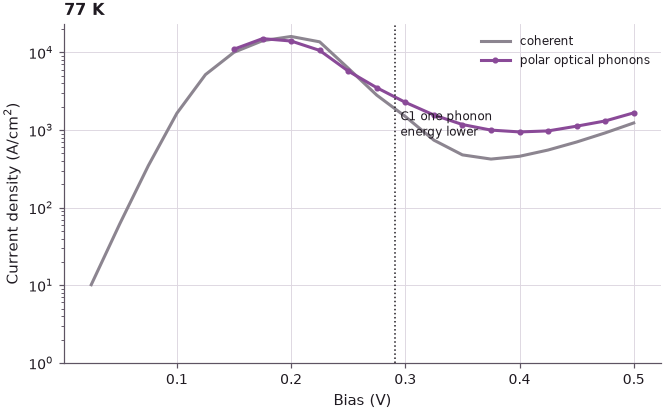
The phonons lower the peak by 6 % and move it to 0.175 V, and add a phonon-assisted current in the valley. Its excess over the coherent current is largest at 0.325 V, just beyond the bias (0.291 V) at which C1 has dropped by one phonon energy below its position at the coherent peak: that is the echo of the main peak, the electrons now entering the well by emitting an LO phonon. In the valley the phonons raise the current by up to a factor of 2.5 (at 0.350 V) and lower the PVR from 38 to 16. With 4 nm Al${0.3}$Ga${0.7}$As barriers the coherent valley is already high (electrons pass over and through the thin, low barriers), so the echo shows as a shoulder rather than a separate peak; in the lecture's AlAs devices at 4 K, where the coherent valley current is many orders of magnitude lower, it appears as a clear replica.

4. Interface roughness: why the I–V becomes asymmetric#

A grown interface is not flat. NEMO models a rough interface as one monolayer in which islands of the two materials alternate, with island fraction $x$ (here 0.5) and an exponential autocorrelation of length $\Lambda$; its average potential $x\,\Delta E_c$ belongs to the device Hamiltonian, and the fluctuation scatters electrons elastically between transverse momenta with a strength $x(1-x)\,\Delta E_c^2$. The scattering rate on an interface is proportional to the density of states there. Under bias, the resonant state in the well is pushed against the collector-side interface (the lower potential), so a rough interface on that side scatters strongly, and the same interface on the emitter side scatters weakly. In the experiment the roughness is not the same on both sides of the well: the interface grown on top of the barrier is usually rougher, as STM images of the Texas Instruments/University of Illinois devices showed. Reversing the bias exchanges the roles.

The two devices below have one rough monolayer, at the emitter-side or at the collector-side interface of the well, with $\Lambda = 10$ nm. Since the structure is otherwise symmetric, the device with the rough monolayer on the collector side in forward bias is the same as the device with it on the emitter side in reverse bias. Each is compared with its own coherent current (the same structure with the scattering switched off).

Slide 6: why interface roughness makes the I–V asymmetric — Slide 6. The scattering rate is proportional to the density of states at the scattering interface. The applied bias tilts the density of states toward the lower potential: weak scattering when the rough interface is on the emitter side, strong scattering when it is on the collector side. Left: InP/InGaAs device cross-section and the asymmetric I–V at 77 K.

Code44 lines · cell 14

ir = {}
for side in ("emitter", "collector"):
    dev = make_rtd(side)
    site = int(np.flatnonzero(np.isclose(dev.band_edge, OFFSET / 2))[0])
    tfd = nemo.thomas_fermi_iv(dev, V, T)
    t0 = RoughnessTransport(dev, [], k_max=0.5, num_k=12)
    t1 = RoughnessTransport(
        dev, [InterfaceRoughness(site, correlation_length=10.0, offset=OFFSET)], k_max=0.5, num_k=12
    )
    j0, j1 = [], []
    for v, u in zip(V, tfd["potential"]):
        e = grid(t1, u, v, T)
        j0.append(t0.solve(e, u, MU, MU - v, T)["current_density"])
        j1.append(t1.solve(e, u, MU, MU - v, T)["current_density"])
    ir[side] = dict(dev=dev, site=site, tf=tfd, j0=np.array(j0), j1=np.array(j1), t1=t1)
    r = nemo.resonances(dev, potential=tfd["potential"][k], emax=0.3, reservoir=RES)
    m = int(np.argmin(abs(r["x0"] - wmid)))
    print(
        f"rough {side:9s} side (site {site}): C1 weight on the rough monolayer at {V[k]:.3f} V = "
        f"{r['density'][m][site] / r['density'][m].max():.2f} of its maximum"
    )

for side, d in ir.items():
    ratio = d["j1"][1:] / d["j0"][1:]
    beyond = V[1:] > V[k]
    print(
        f"rough {side:9s}: J_IR / J_coh at {V[1]:.3f} V {ratio[0]:.2f}, at the peak ({V[k]:.3f} V) "
        f"{ratio[k - 1]:.2f}, "
        f"beyond the peak up to {ratio[beyond].max():.2f} at {V[1:][beyond][np.argmax(ratio[beyond])]:.3f} V"
    )

fig, axs = plt.subplots(1, 2, figsize=(11, 4))
for side, c, lab in (
    ("emitter", style.REFERENCE, "rough interface on the emitter side (reverse)"),
    ("collector", style.OPEN_NEMO, "rough interface on the collector side (forward)"),
):
    d = ir[side]
    axs[0].semilogy(V[1:], d["j1"][1:], color=c, lw=2, label=lab)
    axs[0].semilogy(V[1:], d["j0"][1:], color=c, lw=1, ls=":")
    axs[1].plot(V[1:], d["j1"][1:] / d["j0"][1:], color=c, lw=2, label=lab)
axs[0].set(xlabel="Bias (V)", ylabel="Current density (A/cm$^2$)", title="dotted: same device, coherent")
axs[1].axhline(1, color=style.CONTEXT, lw=0.8)
axs[1].set(xlabel="Bias (V)", ylabel="J with roughness / J coherent")
axs[1].legend(fontsize=8);

rough emitter   side (site 102): C1 weight on the rough monolayer at 0.200 V = 0.27 of its maximum
rough collector side (site 119): C1 weight on the rough monolayer at 0.200 V = 0.37 of its maximum
rough emitter  : J_IR / J_coh at 0.025 V 1.11, at the peak (0.200 V) 1.00, beyond the peak up to 1.04 at 0.425 V
rough collector: J_IR / J_coh at 0.025 V 1.11, at the peak (0.200 V) 0.99, beyond the peak up to 1.26 at 0.375 V

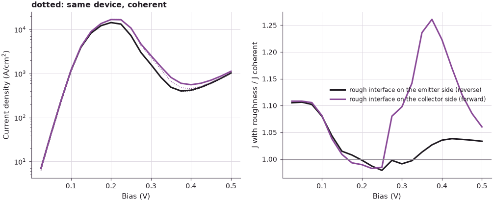
The asymmetry follows the density-of-states argument. At low bias both rough interfaces raise the current by about 10 %, and near the peak they lower it by one or two per cent (the scattering broadens the resonance); beyond the peak the collector-side roughness raises the current by up to 26 %, the emitter-side roughness by at most 4 %. At the peak the resonant state has 0.37 of its maximum weight on the collector-side monolayer and only 0.27 on the emitter-side one. Measured in forward and reverse bias, the same rough interface would thus produce an asymmetric I–V, as on the slide.

5. Alloy disorder and the effective mass: weak effects#

The barrier alloy Al$x$Ga${1-x}$As is random. Each cation site carries a potential fluctuation of $(1-x)\Delta$ or $-x\Delta$ around the virtual-crystal value, with $\Delta \approx 1.08$ eV the GaAs/AlAs $\Gamma$ offset; these are uncorrelated from site to site (ShortRangeScattering.alloy). In the resonator picture this is disorder in the mirrors, which spreads out the resonator spectrum. It is computed here at three biases because each costs about a second.

Code10 lines · cell 16

barrier_sites = np.flatnonzero(rtd.band_edge > OFFSET - 1e-6)
alloy = ShortRangeScattering.alloy(barrier_sites, fraction=x_al, offset=OFFSET / x_al, lattice_constant=0.565)
tra = RoughnessTransport(rtd, [], k_max=0.5, num_k=12, scatterers=[alloy])
for i in (k, kv, len(V) - 1):
    u = tf["potential"][i]
    ja = tra.solve(grid(tra, u, V[i], T), u, MU, MU - V[i], T)["current_density"]
    print(
        f"{V[i]:.3f} V: coherent {J_coh[i]:7.0f} A/cm^2, with alloy disorder {ja:7.0f} A/cm^2 "
        f"({ja / J_coh[i] - 1:+.1%})"
    )

0.200 V: coherent   16064 A/cm^2, with alloy disorder   16135 A/cm^2 (+0.4%)
0.375 V: coherent     423 A/cm^2, with alloy disorder     465 A/cm^2 (+10.0%)
0.500 V: coherent    1235 A/cm^2, with alloy disorder    1295 A/cm^2 (+4.8%)

Alloy scattering changes the peak by well under one per cent and the valley by about ten per cent: a weak effect in GaAs/AlGaAs, as the lecture states. The same holds for the variation of the transverse effective mass between the materials (non-linear media in the optical analogy, which disperse the carriers in the transverse plane): it is already included here through the local mass of each layer and is weak in nearly parabolic GaAs at low temperature.

6. Low temperature against room temperature#

At low temperature, coherent transport in the valley is suppressed and phonon-assisted and roughness-assisted paths dominate. For the AlAs devices of the lecture (slide 9), polar optical phonons and interface roughness raise the valley current by several orders of magnitude and the simulation follows the measured valley at 4 K. At room temperature the picture changes: the thermal distribution of the emitter electrons reaches higher resonances and the tops of the barriers, the coherent valley current rises, and scattering inside the RTD adds comparatively little.

Slide 9: low-temperature I–V with polar optical phonon and interface roughness scattering — Slide 9. Low temperature: polar optical phonon and interface roughness scattering (POP+IR) raise the valley current by several orders of magnitude above the calculation without scattering, and follow the experiment.

Code33 lines · cell 19

T3 = 300
tf3 = nemo.thomas_fermi_iv(rtd, V, T3)
MU3 = float(np.atleast_1d(tf3["mu_left"])[0])
coh3 = RoughnessTransport(rtd, [], k_max=0.8, num_k=16)


def grid3(u, v):
    return energy_grid(coh3, u, MU3, MU3 - v, T3, step=1.5e-3, current_only=True, resonances="on")


J3 = np.array(
    [coh3.solve(grid3(u, v), u, MU3, MU3 - v, T3)["current_density"] for v, u in zip(V, tf3["potential"])]
)
k3 = next(i for i in range(1, len(V) - 1) if J3[i] >= J3[i - 1] and J3[i] > J3[i + 1])  # first local maximum
kv3 = k3 + int(np.argmin(J3[k3:]))
print(
    f"300 K coherent: peak {J3[k3]:.0f} A/cm^2 at {V[k3]:.3f} V, valley {J3[kv3]:.0f} A/cm^2 at "
    f"{V[kv3]:.3f} V, "
    f"PVR {J3[k3] / J3[kv3]:.1f}"
)
for i in (k3, kv3):
    u = tf3["potential"][i]
    jp = coh3.solve_phonon_current(grid3(u, V[i]), u, MU3, MU3 - V[i], T3, pop)["current_density"]
    print(f"300 K, {V[i]:.3f} V: coherent {J3[i]:7.0f}, with POP {jp:7.0f} A/cm^2 ({jp / J3[i] - 1:+.0%})")
i77 = int(np.flatnonzero(VP == V[kv])[0])
print(f"77 K, {V[kv]:.3f} V (coherent valley): with POP {J_pop[i77] / J_coh[kv] - 1:+.0%}")

fig, ax = plt.subplots(figsize=(7, 4))
ax.semilogy(V[1:], J_coh[1:], color=style.CONTEXT, lw=2, label="77 K coherent")
ax.semilogy(VP, J_pop, "--", color=style.CONTEXT, lw=1.5, label="77 K with POP")
ax.semilogy(V[1:], J3[1:], color=style.OPEN_NEMO, lw=2, label="300 K coherent")
ax.set(xlabel="Bias (V)", ylabel="Current density (A/cm$^2$)")
ax.legend(fontsize=8);

300 K coherent: peak 15334 A/cm^2 at 0.200 V, valley 3010 A/cm^2 at 0.325 V, PVR 5.1
300 K, 0.200 V: coherent   15334, with POP   13928 A/cm^2 (-9%)
300 K, 0.325 V: coherent    3010, with POP    4474 A/cm^2 (+49%)
77 K, 0.375 V (coherent valley): with POP +136%

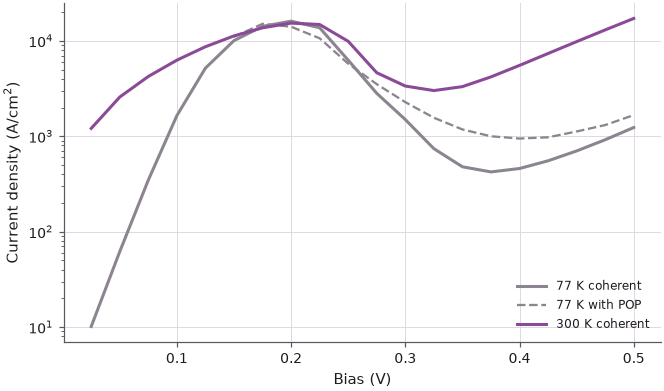
At 300 K the coherent valley current is seven times higher than at 77 K (3010 against 423 A/cm$^2$) and the PVR drops from 38 to 5.1, without any scattering. The polar optical phonons lower the room-temperature peak by 9 % and raise the valley by 49 %, against 136 % at the 77 K valley bias: their relative effect shrinks as the thermal coherent current grows. In this low-barrier test device the phonons still matter at 300 K. The lecture makes the stronger point for its measured room-temperature devices: there the thermal current over and through the barriers dominates the valley, and scattering inside the RTD alone does not reproduce the measured valley or the turn-on of the current beyond it.

Slide 10: at room temperature scattering inside the RTD is not the answer — Slide 10. Measured I–V of an RTD at 77 K, 4.2 K and 300 K. Scattering is important at low temperature and for "physicist devices"; it does not explain the valley current of high-performance devices at room temperature.

7. Scattering in the contacts and the band structure#

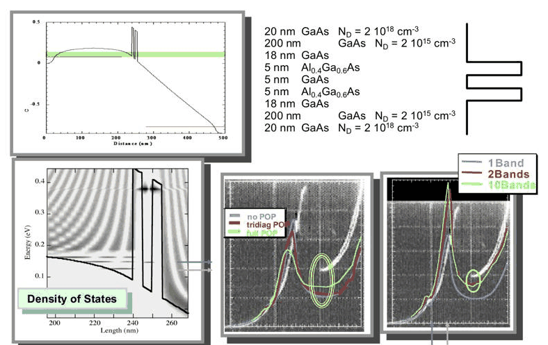
What does explain the room-temperature valley current? NEMO's answer (slide 12) is the treatment of the contacts and of the band structure. Scattering in the reservoirs fills the notch states of the emitter and lets electrons enter at energies below the contact band edge (lecture 11.3), and the full polar-optical-phonon self-energy in the contacts changes the current noticeably compared with no POP or a tridiagonal approximation. Equally important is the band structure: a single-band effective-mass model overestimates the barrier attenuation at high energies, where the real complex band structure (2-band and 10-band models, non-parabolicity) gives lighter imaginary masses and more transmission, and so a higher valley current and an earlier turn-on. These topics are the subject of the band-structure lectures and of the multiband RTD notebooks listed below.

Slide 12: scattering in the contacts and band structure as the sources of valley current — Slide 12. Where the valley current comes from at room temperature: scattering in the contacts (no POP, tridiagonal POP, full POP), which fills the emitter density of states, and the band structure (1-band, 2-band and 10-band models).

8. Exploration: the roughness correlation length#

The strength of interface roughness scattering depends on the lateral size of the islands: a short correlation length $\Lambda$ spreads the scattering over a wide range of transverse momenta, a long one concentrates it on nearby momenta, where scattering changes the state little. The cell repeats the collector-side roughness at the valley bias for several correlation lengths. A finer $k$ grid would be needed for $\Lambda$ much longer than $2\pi/k_\text{max}$.

Code9 lines · cell 25

d = ir["collector"]
u = d["tf"]["potential"][kv]
e = grid(d["t1"], u, V[kv], T)
for lam in (2.0, 5.0, 10.0, 20.0, 40.0):
    trl = RoughnessTransport(
        d["dev"], [InterfaceRoughness(d["site"], correlation_length=lam, offset=OFFSET)], k_max=0.5, num_k=12
    )
    jl = trl.solve(e, u, MU, MU - V[kv], T)["current_density"]
    print(f"Lambda = {lam:4.0f} nm: J = {jl:6.0f} A/cm^2, {jl / d['j0'][kv]:.2f} x coherent ({V[kv]:.3f} V)")

Lambda =    2 nm: J =    549 A/cm^2, 1.15 x coherent (0.375 V)
Lambda =    5 nm: J =    602 A/cm^2, 1.27 x coherent (0.375 V)
Lambda =   10 nm: J =    600 A/cm^2, 1.26 x coherent (0.375 V)
Lambda =   20 nm: J =    576 A/cm^2, 1.21 x coherent (0.375 V)
Lambda =   40 nm: J =    553 A/cm^2, 1.16 x coherent (0.375 V)

The valley current is raised most for correlation lengths of 5–10 nm (by 27 % and 26 %) and less for both shorter and longer ones (15 % at 2 nm, 16 % at 40 nm): long islands scatter almost only forward, into nearly the same state, and very short ones spread the same strength over transverse momenta up to $1/\Lambda$, beyond most of the occupied states. NEMO's comparisons with experiment used correlation lengths of this order, in line with STM images of the interfaces.

Summary#

The valley current of an RTD has several possible sources: incoherent scattering inside the device, scattering in the contacts, and band-structure effects beyond the single-band model.
Phonons act like a vibrating mirror of the resonator: the polar optical phonon (36 meV in GaAs) produces a phonon-assisted current with an echo of the peak in the valley. Its Fröhlich coupling is long-ranged, so its self-energy is a full matrix.
Interface roughness scatters in proportion to the density of states at the rough interface; bias pushes the resonant state against the collector-side interface, so one rough interface gives an asymmetric I–V.
Alloy disorder and transverse-mass effects are weak in GaAs/AlGaAs.
Scattering inside the RTD matters most for the valley at low temperature; at room temperature the coherent valley current grows strongly with the thermal distribution and the relative effect of scattering shrinks (here from +136 % to +49 % in the valley). For the lecture's high-performance devices the contacts and the band structure, not internal scattering, are critical.

Exercises#

Repeat the polar optical phonon calculation at 4.2 K. Does the echo become sharper, and how does the coherent valley current change?
Make the barriers 6 nm thick and recompute the coherent and POP currents at 77 K. How does the ratio of phonon-assisted to coherent valley current change, and why?
Put rough monolayers at both well interfaces. Is the I–V still asymmetric? Compare with the two single-interface cases.
Double num_k and halve the energy step for one bias of each mechanism and estimate the numerical error of the currents quoted here.