

Lecture 2
Challenges at the frontier of quantum transport modeling (NEMO and nanoHUB)
In the lecture
- a 30-year journey: from the first NEMO at Texas Instruments (1994) through NEMO-1D, NEMO3D, NEMO3D-peta, OMEN and NEMO5 to atomistic device modeling used by Intel
- the challenges: modeling that predicts rather than describes, the right basis set, partitioning of an open system, scalable computing, and usability
- devices have become atomically small (a 5 nm node is about 40 atoms long) while TCAD tools stayed atom-agnostic; NEGF as the unified framework from diffusive to quantum transport
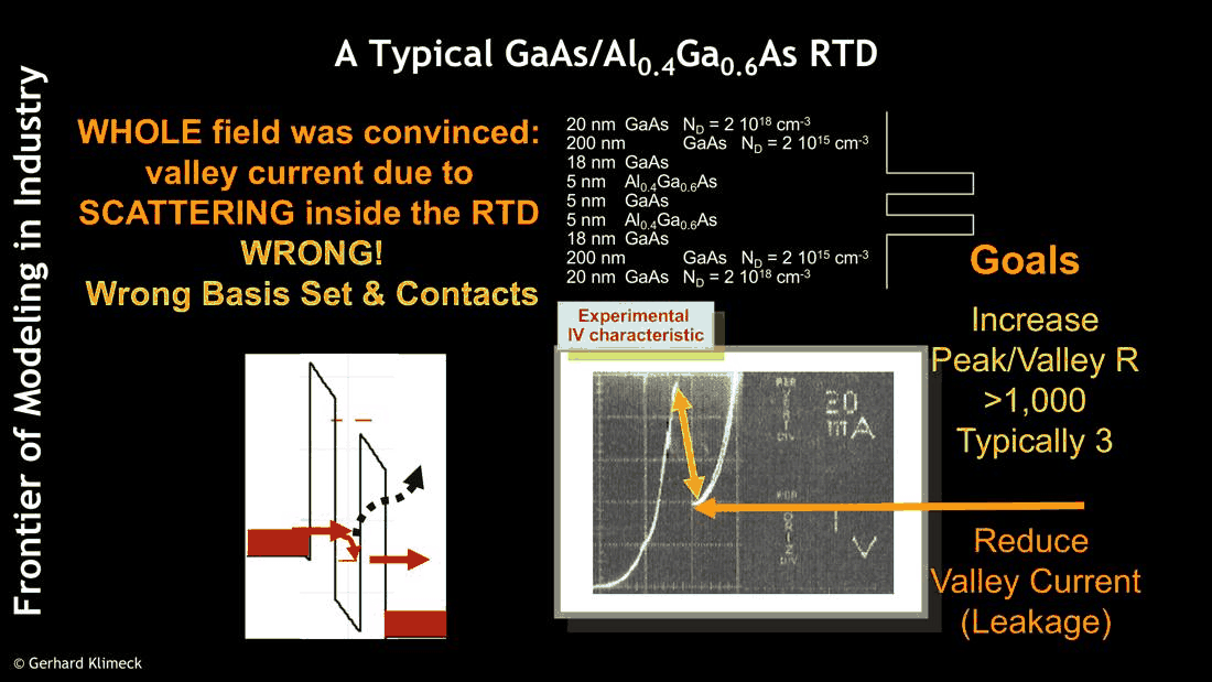
- resonant tunneling diodes: the valley current was blamed on scattering, but came from the band structure and the contacts; modeling exact enough to find growers off by 2 monolayers
- nanowires: the effective mass is not a bulk property, it depends on orientation and confinement
- NEMO generations, the Gordon Bell prize, and nanoHUB as "a new instrument"
In this notebook
we compute small versions of the lecture's key results with open-nemo: the atom counts of the technology nodes; a non-equilibrium Green's function calculation written out by hand and compared with open-nemo's transport solver; the GaAs/AlGaAs RTD of slide 29 at 300 K and 77 K, with the energy-resolved valley current and the effect of 2 monolayers of well width; and the transport masses of 2.1 nm silicon nanowires in three orientations with two tight-binding models, against the values on slide 40.
Run it on your own machine
The notebook needs open-nemo (Python ≥ 3.10 and a C++20 compiler; BLAS/LAPACK).
git clone https://github.com/denphi/open-nemo.git && cd open-nemo
python3 -m venv .venv && source .venv/bin/activate
pip install -e ".[notebooks]"
jupyter lab From_Atoms_to_Devices/01_introduction/02_0_frontier_of_quantum_transport.ipynbCode
import numpy as np
import matplotlib.pyplot as plt
import opennemo as nemo
from opennemo.visualization import style

style.use(notebook=True)
from opennemo.structures import lattice
from opennemo.structures.energy import resonance_finder

KB = nemo.core.units.KB
H2M0 = nemo.core.units.HBAR2_2M0
1. A 30-year journey, and devices counted in atoms#
Klimeck's journey starts at Texas Instruments, where NEMO (NanoElectronic MOdeling) was presented in 1995 as a tool to design resonant tunneling devices. Its successors followed the devices: NEMO-1D (TI 1994–98, JPL 1998–2003), NEMO3D (JPL and Purdue, 1998–2007) for quantum dots of millions of atoms, NEMO3D-peta (2006–11), OMEN (M. Luisier, ETH Zürich and Purdue, from 2006) for full-band atomistic transport in transistors, and NEMO5 (Purdue, from 2009). The challenges have stayed the same: models must predict, not describe; the basis set must be right; the open system must be partitioned into contacts and device; the computation must scale; and the tools must be usable by others.
Slide 11 recalls the 2009 Intel roadmap with nodes of 22, 14, 10, 7 and 5 nm, about 176, 122, 80, 56 and 40 atoms long, while "all TCAD tools are atom-agnostic". The count depends on the spacing of atomic planes along the channel, which open-nemo's silicon crystal gives for the common directions.
Code
si = nemo.structures.materials.load("boykin2004_sp3d5s")["Si"]
a = si.lattice_constant
spacing = {"[001] (a/4)": a / 4, "[110] (a√2/4)": a * np.sqrt(2) / 4,
           "[111] (a√3/4, mean)": a * np.sqrt(3) / 4}
slide = {22: 176, 14: 122, 10: 80, 7: 56, 5: 40}
print(f"Si: a = {a:.4f} nm;  plane spacings " + ", ".join(f"{k} {v:.4f} nm" for k, v in spacing.items()))
print(" node (nm)  slide  " + "  ".join(f"{k:>18s}" for k in spacing))
for node, n in slide.items():
    print(f"{node:9d}  {n:5d}  " + "  ".join(f"{node / d:18.0f}" for d in spacing.values()))
print(f"spacing implied by the slide: {np.mean([k / v for k, v in slide.items()]):.3f} nm per atom")
Si: a = 0.5431 nm;  plane spacings [001] (a/4) 0.1358 nm, [110] (a√2/4) 0.1920 nm, [111] (a√3/4, mean) 0.2352 nm
 node (nm)  slide         [001] (a/4)       [110] (a√2/4)  [111] (a√3/4, mean)
       22    176                 162                 115                  94
       14    122                 103                  73                  60
       10     80                  74                  52                  43
        7     56                  52                  36                  30
        5     40                  37                  26                  21
spacing implied by the slide: 0.123 nm per atom
The slide's counts correspond to about 0.123 nm per atom, close to the \(a/4 = 0.136\) nm spacing of atomic planes along [001]; along [110] the same lengths hold about 30 % fewer planes. Either way, a 5 nm channel holds a few dozen atomic planes, and a fin about 6 nm wide (TSMC's 5 nm technology, IEDM 2019) about 48 atoms across. Classical clock-speed scaling stopped around 2005, but the devices kept shrinking; Moore's law was declared dead many times and was not.
2. Which formalism? NEGF and the partitioning of open systems#
Transport can be described at many levels: drift–diffusion (Lecture 1.4), the Boltzmann equation for distributions of particles, and quantum transport, where the wave nature of the electrons matters. The non-equilibrium Green's function (NEGF) formalism, developed from the work of Schwinger, Kadanoff and Baym, and Keldysh, and brought to devices by Datta, Lake and others, contains them all: ballistic and diffusive transport, coherent and incoherent, in one framework. Klimeck calls one of its features "the most underappreciated": the spatial partitioning of an open system. The contacts, semi-infinite, enter only through self-energies \(\Sigma_1\), \(\Sigma_2\) at the boundary of a finite device; scattering enters through another self-energy \(\Sigma_s\).
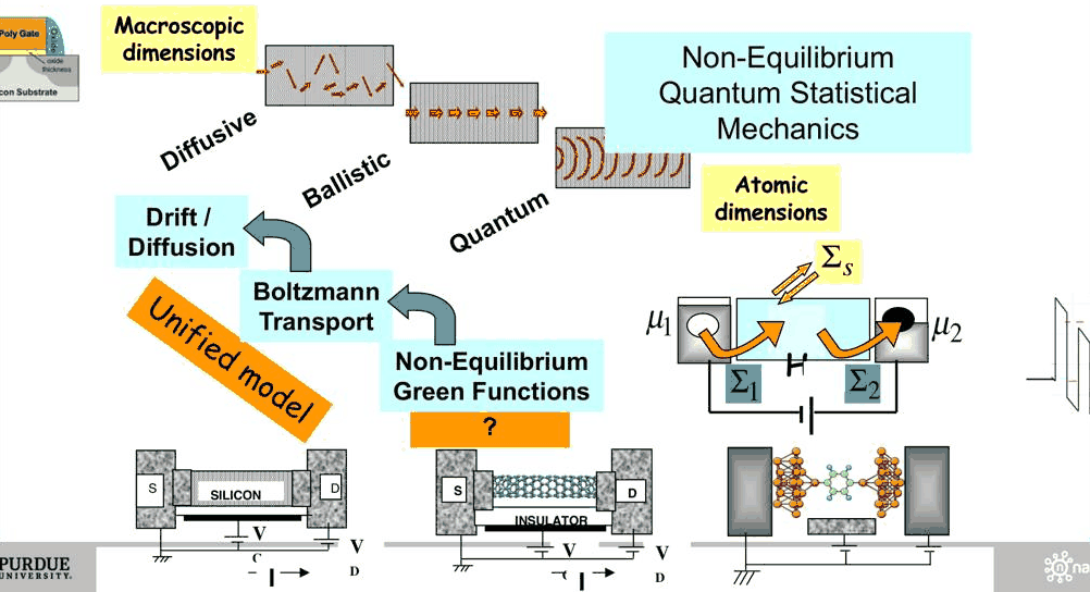
The whole method fits in a few lines for a one-dimensional effective-mass device. The Hamiltonian on a grid of spacing \(\Delta\) is tridiagonal, with hopping \(t = -\hbar^2/2m^*\Delta^2\). A lead of on-site energy \(\varepsilon\) carries waves of energy \(E = \varepsilon + 2t\cos(k\Delta)\), and its self-energy on the adjacent device site is \(\Sigma = t\,e^{ik\Delta}\). Then
The cell builds the GaAs/Al${0.4}$Ga${0.6}$As double barrier of slide 29 (5 nm barriers, a 5 nm
well), takes open-nemo's Hamiltonian matrix, and compares this hand-made NEGF with open-nemo's
Transport.
Code
gaas = nemo.structures.materials.effective_mass("GaAs")
algaas = nemo.structures.materials.effective_mass("AlGaAs", x=0.4)
dbl = nemo.Heterostructure1D([nemo.Layer(gaas, 10), nemo.Layer(algaas, 5), nemo.Layer(gaas, 5),
                              nemo.Layer(algaas, 5), nemo.Layer(gaas, 10)], spacing=0.1)
h = dbl.hamiltonian.sparse.matrices[0].toarray().real    # the device Hamiltonian (eV), closed
eps, t = h[0, 0], h[0, 1]                                  # lead on-site energy and hopping
print(f"{h.shape[0]} sites; lead: eps = {eps:.4f} eV, t = {t:.4f} eV "
      f"(-ħ²/2m*Δ² = {-H2M0 / (gaas.mass * 0.1**2):.4f} eV)")


def negf_transmission(energy):
    ka = np.arccos((energy - eps) / (2 * t) + 0j)          # lead dispersion E = eps + 2t cos(ka)
    sigma = t * np.exp(1j * ka)
    if sigma.imag > 0:                                     # pick the retarded (outgoing) solution
        sigma = np.conj(sigma)
    n = h.shape[0]
    s1, s2 = np.zeros((n, n), complex), np.zeros((n, n), complex)
    s1[0, 0], s2[-1, -1] = sigma, sigma
    g = np.linalg.inv(energy * np.eye(n) - h - s1 - s2)
    g1, g2 = 1j * (s1 - s1.conj().T), 1j * (s2 - s2.conj().T)
    return np.trace(g1 @ g @ g2 @ g.conj().T).real


res = nemo.resonances(dbl)
e_test = np.array([0.02, 0.05, res["energy"][0], 0.15, 0.25, 0.40])
t_nemo = nemo.Transport(dbl.hamiltonian).transmission(e_test)
print("   E (eV)    T by hand      T open-nemo    relative difference")
for e, tn in zip(e_test, t_nemo):
    th = negf_transmission(e)
    print(f"{e:9.4f}   {th:12.4e}   {tn:12.4e}   {abs(th - tn) / tn:10.1e}")
print(f"first resonance E_1 = {1e3 * res['energy'][0]:.2f} meV, width {1e6 * res['width'][0]:.1f} µeV")
350 sites; lead: eps = 113.7308 eV, t = -56.8654 eV (-ħ²/2m*Δ² = -56.8654 eV)
   E (eV)    T by hand      T open-nemo    relative difference
   0.0200     7.3123e-09     7.3123e-09      4.7e-07
   0.0500     1.8738e-07     1.8738e-07      1.1e-07
   0.0822     1.0000e+00     1.0000e+00      9.7e-11
   0.1500     6.3056e-06     6.3056e-06      3.7e-08
   0.2500     4.6416e-04     4.6416e-04      5.4e-09
   0.4000     1.2130e-01     1.2130e-01      2.3e-08
first resonance E_1 = 82.25 meV, width 63.9 µeV
The two agree to better than one part in a million, including on the first resonance, where the transmission reaches one. open-nemo's solver does the same thing more cleverly (recursive Green's functions, leads with many modes, atomistic bases), but the physics is these few lines: a finite device, two self-energies, one inverse. The self-energies are the reason a calculation of a device of a few thousand atoms can describe a circuit with infinite wires attached.
3. Resonant tunneling diodes: the valley current and the basis set#
Slide 29 describes the device that started it: a GaAs/Al${0.4}$Ga${0.6}$As RTD with 5 nm barriers and a 5 nm well, 18 nm undoped spacers and contacts doped \(2\times10^{18}\) cm⁻³. The goal of the TI project was to reduce the valley current, the current beyond the peak that spoils the peak-to-valley ratio. The whole field believed that the valley current came from scattering. That was wrong: what was missing was the right basis set (band structure) and the right treatment of the contacts. Slide 33 sums up: the valley current comes from thermionic emission into excited states and from tunneling through the band structure, so the peak-to-valley ratio is fundamentally limited even without scattering.
The cell computes the ballistic current of this device in the effective-mass approximation: the
bias drops linearly between the ends of the spacers, the transmission is computed on an energy grid
that resonance_finder refines around the narrow resonances, and the current density follows from
the Tsu–Esaki integral over the Fermi functions of the two contacts. There is no scattering in this
model.
Code
def rtd(well=5.0, barrier=5.0):
    layers = [nemo.Layer(gaas, 20, donors=2e18), nemo.Layer(gaas, 18), nemo.Layer(algaas, barrier),
              nemo.Layer(gaas, well), nemo.Layer(algaas, barrier), nemo.Layer(gaas, 18),
              nemo.Layer(gaas, 20, donors=2e18)]
    return nemo.Heterostructure1D(layers, spacing=0.1)


def iv(dev, volts, temp=300.0, spectrum_at=None):
    mu = dev.contact_fermi_level("left", temp)
    frac = np.clip((dev.x - 20.0) / (dev.x[-1] - 40.0), 0, 1)     # linear drop between the doped regions
    tr, kt, cur, spec = nemo.Transport(dev.hamiltonian), KB * temp, [], None
    for v in volts:
        u = -v * frac
        e, tt = resonance_finder(lambda en: tr.transmission(en, potential=u), -v + 1e-4,
                                 mu + 25 * kt + 0.05, n0=300)
        cur.append(dev.current_density(e, tt, mu, mu - v, temp))
        if spectrum_at is not None and np.isclose(v, spectrum_at):
            fl, fr = 1 / (1 + np.exp((e - mu) / kt)), 1 / (1 + np.exp((e - mu + v) / kt))
            spec = (e, tt * (fl - fr))
    return np.array(cur), mu, spec


def peak_valley(volts, cur):
    i = next(k for k in range(1, len(cur) - 1) if cur[k] > cur[k - 1] and cur[k] >= cur[k + 1])
    j = i + int(np.argmin(cur[i:i + 8]))
    return i, j


volts = np.round(np.arange(0.0, 0.601, 0.02), 3)
dev = rtd()
fig, (ax1, ax2) = plt.subplots(1, 2, figsize=(11, 4))
results = {}
for c, temp in zip((style.OPEN_NEMO, style.REFERENCE), (300.0, 77.0)):
    cur, mu, _ = iv(dev, volts, temp)
    i, j = peak_valley(volts, cur)
    results[temp] = (cur, i, j)
    ax1.semilogy(volts, np.maximum(cur, 1e-3), "o-", ms=3, color=c, label=f"{temp:.0f} K")
    print(f"{temp:5.0f} K: E_F = {1e3 * mu:.1f} meV; peak {cur[i]:.0f} A/cm² at {volts[i]:.2f} V, "
          f"valley {cur[j]:.3g} A/cm² at {volts[j]:.2f} V, PVR {cur[i] / cur[j]:.1f}")
ax1.set(xlabel="bias V (V)", ylabel="current density J (A/cm²)")
ax1.legend(fontsize=8)

# where in energy does the 300 K valley current flow?
i, j = results[300.0][1:]
for c, v, name in ((style.sweep(2)[0], volts[i], "peak"), (style.sweep(2)[1], volts[j], "valley")):
    _, mu, (e, s) = iv(dev, [v], 300.0, spectrum_at=v)
    s = np.maximum(s, 0)
    ax2.semilogx(np.maximum(s, 1e-16), e, color=c, label=f"{name}, V = {v:.2f} V")
    mean = np.trapezoid(e * s, e) / np.trapezoid(s, e)
    hot = np.trapezoid(s[e > mu + 3 * KB * 300], e[e > mu + 3 * KB * 300]) / np.trapezoid(s, e)
    print(f"{name} (V = {v:.2f} V): mean energy of the current {1e3 * mean:.0f} meV above the emitter "
          f"band edge; {100 * hot:.0f} % from electrons more than 3 kT above E_F")
ax2.axhline(mu, color=style.CONTEXT, ls="--", lw=1)
ax2.set(xlabel=r"$T(E)\,[f_L - f_R]$", ylabel="energy E (eV, emitter band edge = 0)", xlim=(1e-14, 1))
ax2.legend(fontsize=8)
fig.tight_layout()
  300 K: E_F = 79.1 meV; peak 8987 A/cm² at 0.16 V, valley 1.43e+03 A/cm² at 0.18 V, PVR 6.3
   77 K: E_F = 86.0 meV; peak 9058 A/cm² at 0.14 V, valley 30.6 A/cm² at 0.20 V, PVR 295.6
peak (V = 0.16 V): mean energy of the current 65 meV above the emitter band edge; 28 % from electrons more than 3 kT above E_F
valley (V = 0.18 V): mean energy of the current 214 meV above the emitter band edge; 98 % from electrons more than 3 kT above E_F
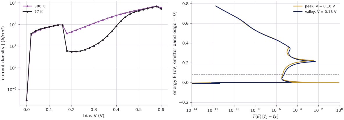
Even without any scattering the current falls after the peak by a finite factor: the peak-to-valley ratio is 6.3 at 300 K. Cooling to 77 K raises it to about 300, because the valley current at 300 K is carried by hot electrons. At the peak most of the current flows through the first resonance, which the bias has pulled down close to the emitter band edge, inside the Fermi sea (mean energy 65 meV, below \(E_F\) = 79 meV). At the valley that resonance lies below the band edge, and 98 % of the current comes from the thermal tail more than \(3k_BT\) above \(E_F\), through the second resonance near 0.2 eV and over the barriers (right panel; mean energy 214 meV). This is the "thermionic emission into excited states" of slide 33. In real devices tunneling through the band structure adds to it — X-valley states of AlGaAs, non-parabolicity — which only a full-band model such as NEMO's tight binding (Lecture 1.3) describes.
4. Modeling exact to a monolayer#
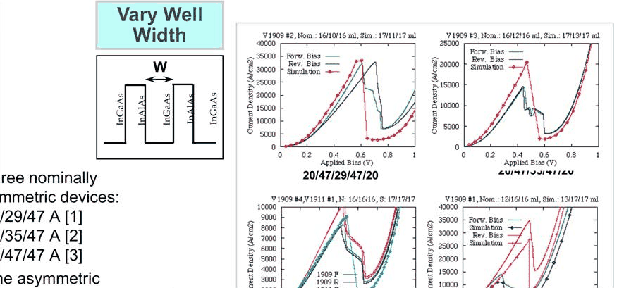
The next test of NEMO came from InGaAs/InAlAs RTDs grown on InP: four stacks with nominal well widths of 47/29/47, 47/35/47, 47/47/47 and an asymmetric 35/47/47 Å. With the full band structure the simulations matched the measured current–voltage curves — once the well and barrier widths were taken 2 monolayers thicker than nominal. "Modeling was exact! Growers were off by 2 monolayers consistently! They corrected their growth recipes!"
How large is the effect of 2 monolayers? In GaAs a monolayer is \(a/2 = 0.283\) nm, so 2 ML are 0.57 nm; on the 0.1 nm grid of the model the well changes by ±0.6 nm.
Code
ml = nemo.structures.properties.value("GaAs", "lattice_constant") / 2
print(f"1 ML of GaAs = {ml:.4f} nm, 2 ML = {2 * ml:.3f} nm")
print(" well (nm)   E_1 (meV)   peak bias (V)   peak J (A/cm²)")
fig, ax = plt.subplots(figsize=(6.5, 3.8))
for c, w in zip(style.sweep(3), (4.4, 5.0, 5.6)):
    d = rtd(well=w)
    bare = nemo.Heterostructure1D([nemo.Layer(gaas, 10), nemo.Layer(algaas, 5), nemo.Layer(gaas, w),
                                   nemo.Layer(algaas, 5), nemo.Layer(gaas, 10)], spacing=0.1)
    e1 = nemo.resonances(bare)["energy"][0]                  # first resonance at zero bias
    cur, _, _ = iv(d, volts)
    i, _ = peak_valley(volts, cur)
    ax.plot(volts, cur, "o-", ms=3, color=c, label=f"well {w:.1f} nm")
    print(f"{w:9.1f}   {1e3 * e1:9.1f}   {volts[i]:13.2f}   {cur[i]:14.0f}")
ax.set(xlabel="bias V (V)", ylabel="current density J (A/cm²)", ylim=(0, 2.5e4))
ax.legend(fontsize=8)
fig.tight_layout()
1 ML of GaAs = 0.2827 nm, 2 ML = 0.565 nm
 well (nm)   E_1 (meV)   peak bias (V)   peak J (A/cm²)
      4.4        95.5            0.18            17736
      5.0        82.2            0.16             8987
      5.6        71.6            0.12             5897
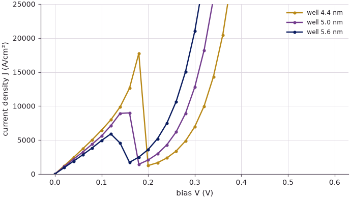
Two monolayers (0.6 nm) move the first resonance by 11–13 meV and the current peak by 0.02–0.04 V, and change the peak current by about a factor of two: easily measurable. Conversely, a model that is right to that level can tell the grower what was grown. This is what Klimeck means by modeling that predicts rather than describes.
5. Nanowires: the effective mass is not a bulk property#
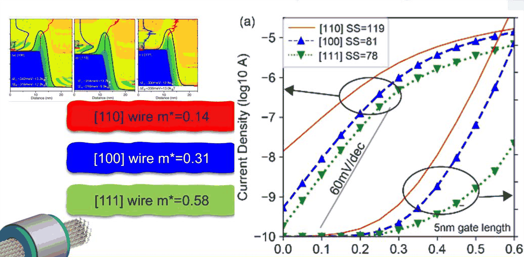
The lecture's second story is the silicon nanowire. Band Structure Lab on nanoHUB (more than 13,000 users) and the OMEN-based omenwire tool compute wires atom by atom. Slide 40 shows a 2.1 nm wire transistor in three orientations, with transport masses of 0.31 \(m_0\) for [100], 0.14 \(m_0\) for [110] and 0.58 \(m_0\) for [111] — different from each other by a factor of four, and different from silicon's bulk masses (0.19 and 0.92 \(m_0\)). "Effective mass is not a bulk property; it can be designed by geometry and strain."
The cell builds hydrogen-passivated 2.1 nm cylindrical Si wires along [100], [110] and [111], computes the band structure of the wire (one period along the axis, all atoms of the cross-section) and takes the transport mass from the curvature of the lowest conduction subband at its minimum, \(m^* = \hbar^2/(\partial^2E/\partial k^2)\). It does so with the sp3d5s* model and with the older sp3s* model, whose conduction band minimum is in the wrong place. The six wires take about half a minute.
Code
def wire_mass(pset, direction, confinement, diameter=2.1):
    mat = nemo.structures.materials.load(pset)["Si"]
    o = lattice.oriented(lattice.from_material(mat), direction, confinement)
    cv = o.conventional
    ny, nz = (int(np.ceil((diameter + 0.6) / cv[k, k])) for k in (1, 2))
    cyl = nemo.structures.shapes.Cylinder(center=[ny * cv[1, 1] / 2, nz * cv[2, 2] / 2],
                                          radius=diameter / 2, axis=0)
    wire = nemo.Device(o, cells=(2, ny, nz), cross_section=cyl)
    ham = nemo.models.tb.SlaterKoster(mat, passivation=30.0).partition(wire)
    ka = np.linspace(0, np.pi, 61)
    bands = np.asarray(ham.lead().bands(ka))
    levels = np.sort(bands[0])
    inner = levels[(levels > -2) & (levels < 3)]
    g = np.argmax(np.diff(inner))
    mid = 0.5 * (inner[g] + inner[g + 1])                   # middle of the gap
    cb = np.array([b[b > mid].min() for b in bands])
    vb = np.array([b[b < mid].max() for b in bands])
    i = int(np.argmin(cb))
    j, dk = min(max(i, 1), len(ka) - 2), (ka[1] - ka[0]) / cv[0, 0]
    curvature = (cb[j + 1] - 2 * cb[j] + cb[j - 1]) / dk**2
    return cb.min() - vb.max(), ka[i] / np.pi, 2 * H2M0 / curvature, ham.num_orbitals   # m* = ħ²/E''


orientations = {"[100]": ([1, 0, 0], [0, 1, 0]), "[110]": ([1, 1, 0], [0, 0, 1]),
                "[111]": ([1, 1, 1], [1, -1, 0])}
slide40 = {"[100]": 0.31, "[110]": 0.14, "[111]": 0.58}
masses = {}
print("model                wire   orbitals/period   gap (eV)   CB min (π/period)   m* (m0)   slide 40")
for pset in ("boykin2004_sp3d5s", "vogl1983_sp3s"):
    for name, (d, c) in orientations.items():
        gap, kmin, m, norb = wire_mass(pset, d, c)
        masses[(pset, name)] = m
        print(f"{pset:19s}  {name}   {norb // 2:15d}   {gap:8.3f}   {kmin:17.2f}   {m:7.3f}   "
              f"{slide40[name]:8.2f}")

fig, ax = plt.subplots(figsize=(6.5, 3.6))
xs = np.arange(3)
ax.bar(xs - 0.25, list(slide40.values()), 0.25, color=style.CONTEXT, label="slide 40 (OMEN)")
ax.bar(xs, [masses[("boykin2004_sp3d5s", n)] for n in orientations], 0.25, color=style.OPEN_NEMO,
       label="open-nemo sp3d5s*")
ax.bar(xs + 0.25, [masses[("vogl1983_sp3s", n)] for n in orientations], 0.25, color=style.REFERENCE,
       label="open-nemo sp3s*")
ax.axhline(0.19, color=style.CONTEXT, ls=":", lw=1)
ax.text(2.45, 0.2, "bulk $m_t$", fontsize=8, ha="right")
ax.set_xticks(xs, list(orientations))
ax.set(xlabel="wire orientation (2.1 nm diameter)", ylabel="transport mass $m^*$ ($m_0$)")
ax.legend(fontsize=8)
fig.tight_layout()
model                wire   orbitals/period   gap (eV)   CB min (π/period)   m* (m0)   slide 40
boykin2004_sp3d5s    [100]               970      1.961                0.00     0.347       0.31
boykin2004_sp3d5s    [110]               660      1.637                0.00     0.141       0.14
boykin2004_sp3d5s    [111]              1520      1.849                0.28     0.540       0.58
vogl1983_sp3s        [100]               485      1.620                0.50     0.771       0.31
vogl1983_sp3s        [110]               330      1.526                0.72     1.288       0.14
vogl1983_sp3s        [111]               760      1.537                0.58     1.571       0.58
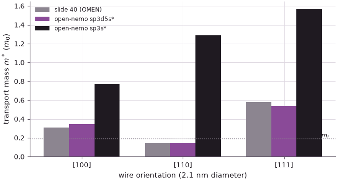
With the sp3d5s* model the three masses come out close to the values on slide 40, in the same order: [110] is the lightest, [111] the heaviest, [100] in between and well above the bulk transverse mass. The [110] wire has the lightest mass and, at a given gate overdrive, the most current — and the strongest source-to-drain tunneling in a short channel, which is why its subthreshold swing on slide 40 is the worst. The sp3s* model, with its conduction minimum at the wrong place in the Brillouin zone, gives masses that are wrong by factors of 2.5 to 9: the choice of basis decides the answer. Geometry, orientation and strain are design parameters for the mass — something no bulk effective-mass model can tell you.
6. Scaling up: NEMO generations and a new instrument#
Each NEMO generation extended what could be computed: NEMO-1D (about 1,000 atoms, the first predictive NEGF tool and the first NEGF tool used in industry), NEMO3D (50 million atoms, the first 10-million-atom electronic structure), NEMO3D-peta (100 million atoms on 30,000 cores), OMEN (about 140,000 atoms in full-band transport on 220,000 cores, a Gordon Bell prize) and NEMO5 (100 million atoms, 200,000 cores), adopted by Intel, Samsung, GlobalFoundries and others. Along the way: oxide thickness metrology at TI (1997), valley splitting in strained Si quantum wells, single-dopant metrology in FinFETs (Nature Physics 2008), a single-phosphorus-atom transistor (2012), and in 2013 the rewriting of the ITRS tables for process integration with NEMO5.
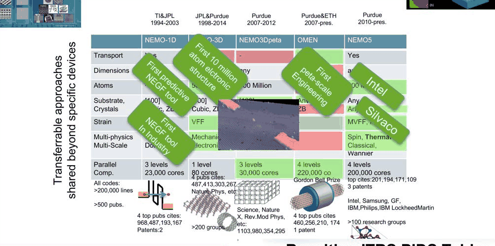
The sizes in the table set the computational problem. A tight-binding basis with 10 orbitals per atom (20 with spin) turns 100 million atoms into a matrix of \(2\times10^9\) rows; the 2.1 nm wires above already need the number of orbitals per period printed in the table. Klimeck closes by comparing nanoHUB and NEMO to a new instrument, like the 100-inch mirror of the Mount Wilson telescope: a tool that lets a community see what it could not see before.
Summary#
- A 5 nm channel is a few dozen atomic planes long (37 along [001]); the slide's node counts correspond to about 0.12 nm per atom.
- NEGF in a few lines — \(G = (E - H - \Sigma_1 - \Sigma_2)^{-1}\), \(T = \mathrm{Tr}[\Gamma_1G\Gamma_2G^\dagger]\) — reproduces open-nemo's transmission to better than \(10^{-6}\); the contacts enter only through the self-energies.
- The GaAs/Al${0.4}$Ga${0.6}$As RTD of slide 29 has, without any scattering, a finite valley current: PVR 6.3 at 300 K and about 300 at 77 K. The 300 K valley current is carried by hot electrons through the excited resonance and over the barriers.
- Two monolayers of well width move the RTD's resonance by 11–13 meV, its current peak by 0.02–0.04 V, and its peak current by about a factor of two.
- The transport masses of 2.1 nm Si wires from sp3d5s* tight binding follow slide 40 ([110] lightest, [111] heaviest); sp3s* gets them wrong.
Exercises#
- Add a Büttiker-probe-like broadening by giving the hand-made NEGF a small imaginary energy, \(E \to E + i\eta\). How does the first resonance's peak transmission change with \(\eta\) = 10, 100, 1000 µeV? Compare \(\eta\) with the resonance width.
- Repeat the RTD calculation with 4 nm and 6 nm barriers. How do the peak current and the peak-to-valley ratio at 300 K change?
- Compute the [100] and [110] wire masses for diameters of 1.5, 2.1 and 3 nm with sp3d5s*. Do they approach the bulk values?
- The slide quotes 176 atoms for 22 nm. Which plane spacing would give exactly this, and which crystal direction comes closest?
Further reading#
- RTD tutorial
- RTD scattering
- Atomistic against effective-mass RTD
- Wire direction and cross-section
- Benchmarks: NEMO-1D default RTD, Bowen et al. 1997 RTD, NEMO3D, Klimeck 2002, OMEN nanowires
- G. Klimeck, R. Lake, R. C. Bowen, W. R. Frensley and T. S. Moise, "Quantitative simulation of a resonant tunneling diode", Appl. Phys. Lett. 67, 2539 (1995).
- R. C. Bowen, G. Klimeck, R. K. Lake, W. R. Frensley and T. Moise, "Quantitative simulation of a resonant tunneling diode", J. Appl. Phys. 81, 3207 (1997).
- R. Lake, G. Klimeck, R. C. Bowen and D. Jovanovic, "Single and multiband modeling of quantum electron transport through layered semiconductor devices", J. Appl. Phys. 81, 7845 (1997).
- M. Luisier, A. Schenk, W. Fichtner and G. Klimeck, "Atomistic simulation of nanowires in the sp3d5s* tight-binding formalism", Phys. Rev. B 74, 205323 (2006).
- S. Datta, Quantum Transport: Atom to Transistor (Cambridge University Press, 2005).