Lecture 11.1

Introduction to resonant tunneling diodes — RTDs with linear potential drops

In the lecture

a reminder of double-barrier tunneling: unity transmission below the barrier top, resonance widths set by the barriers
how a resonant tunneling diode (RTD) works: the ground state is an energy bandpass filter that is pulled through the electron supply of the emitter, which gives an N-shaped current–voltage (I–V) curve with negative differential resistance
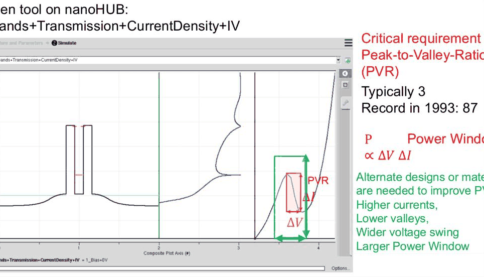
the peak-to-valley current ratio (PVR) and the power window as the figures of merit
a GaAs/Al${0.3}$Ga${0.7}$As RTD with an assumed linear potential drop: transmission, energy-resolved current density and its running integral at 0, 0.08 and 0.16 V
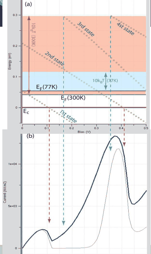
resonance energies and widths as functions of bias, turn-on and turn-off voltages at 77 K and 300 K, and how much of the current each resonance carries

In this notebook

builds the lecture's RTD (7 nm GaAs well, 5 nm Al${0.3}$Ga${0.7}$As barriers) with a linear potential drop, computes its transmission $T(E)$, the current density spectrum $J(E)$ and its running integral, tracks the resonance energies and widths against bias, computes the I–V curves at 77 K and 300 K with the Tsu–Esaki formula, splits the current among the resonances, and explores how the barrier thickness changes the peak current and the peak-to-valley ratio.

Run the notebookEvery number and figure on this page comes from it. Change it, rerun it, take it further.

Download .ipynb View on GitHub

Run it on your own machine

The notebook needs open-nemo (Python ≥ 3.10 and a C++20 compiler; BLAS/LAPACK).

git clone https://github.com/denphi/open-nemo.git && cd open-nemo
python3 -m venv .venv && source .venv/bin/activate
pip install -e ".[notebooks]"
jupyter lab From_Atoms_to_Devices/06_resonant_tunneling_diodes/11_1_rtds_with_linear_potential_drops.ipynb

Code8 lines · cell 1

import numpy as np
import matplotlib.pyplot as plt
import opennemo as nemo
from opennemo.visualization import style

style.use(notebook=True)
H2M0 = nemo.core.units.HBAR2_2M0          # ħ²/2m₀ = 0.0381 eV nm²
EM = nemo.structures.materials.EffectiveMassMaterial

1. Reminder: resonant tunneling through a double barrier#

The previous section showed that a double barrier transmits electrons with probability one at certain energies below the barrier height. Between the two barriers the electron sees a well; at the energies of the quasi-bound states of that well the waves reflected from the two barriers cancel, and the transmission coefficient $T(E)$ reaches 1 (for symmetric barriers). Above the barriers there are weaker resonance features as well. Higher and thicker barriers keep the electron in the well for longer: the resonance lifetime $\tau$ grows and the resonance width $\Gamma = \hbar/\tau$ shrinks. Close to an isolated resonance at $E_0$ the transmission has the Breit–Wigner (Lorentzian) shape

T(E) \approx \frac{\Gamma_L\Gamma_R}{(E-E_0)^2 + (\Gamma_L+\Gamma_R)^2/4},

where $\Gamma_L$ and $\Gamma_R$ are the partial widths for escape through the left and the right barrier and $\Gamma=\Gamma_L+\Gamma_R$ is the full width at half maximum. For a symmetric structure $\Gamma_L=\Gamma_R$ and the peak value is 1.

This lecture puts such a double barrier between two doped contacts and asks what current flows when a voltage is applied.

2. How a resonant tunneling diode works#

The emitter (left contact) is doped, so its conduction band is filled with electrons up to the Fermi level $E_F$: a "sea of electrons" a few tens of meV deep. The well holds a quasi-bound state that at zero bias lies somewhat above $E_F$. An applied voltage pulls the right side of the structure down, and with it the resonance. The sequence that follows is drawn on the slide:

Turn-on. The resonance enters the thermally occupied energy range of the emitter and electrons at its energy can pass. The current grows as the resonance moves deeper into the sea.
Peak. The resonance acts as an energy bandpass filter: the current is largest when the filter is aligned with the best-supplied part of the emitter. How large it is depends on the resonance width and on the electron supply.
Valley. Further bias pulls the resonance below the emitter conduction band edge. There are no emitter electrons at that energy any more; the current falls although the voltage rises. This is negative differential resistance (NDR).
Second turn-on. The next, excited resonance comes down into the sea and the current rises again.

The result is an N-shaped I–V characteristic. The NDR region makes RTDs candidates for very high frequency oscillators (THz) and for compact logic and memory circuits.

Slide 10: schematic I–V curve of an RTD with the band diagrams at turn-on, peak, valley and second turn-on — Slide 10. The ground state (green) and the first excited state (orange) are pulled through the electron sea of the emitter. Peak current at alignment, valley current when the ground state is below the emitter band edge, and a second rise when the excited state arrives.

The quantity that matters for applications is the peak-to-valley current ratio (PVR), the peak current divided by the following valley current. Typical devices reach a PVR of about 3; the record quoted on the slide (from 1993) is 87. Applications need much more, of the order of 1000. A second figure of merit is the power window: the voltage swing $\Delta V$ times the current swing $\Delta I$ of the NDR region, which sets the power an RTD oscillator can deliver. Higher currents, lower valleys, a wider voltage swing all ask for better designs or better materials, and finding them is what device modeling is for. The lecture uses the nanoHUB tool RTDnegf, which runs the simulation engine of NEMO-1D in the background and plots bands, transmission, current density and the I–V curve side by side.

Slide 11: the RTDnegf tool on nanoHUB, with the peak-to-valley ratio and the power window marked on an I–V curve — Slide 11. RTDnegf on nanoHUB: band diagram with the resonance, transmission, current density and the I–V curve. The red box marks the peak-to-valley ratio, the green box the power window $\propto \Delta V\,\Delta I$.

3. A GaAs/AlGaAs RTD with a linear potential drop#

The lecture's device has a 7 nm GaAs well between two 5 nm Al${0.3}$Ga${0.7}$As barriers, with a conduction band offset $\Delta E_c = 324$ meV. The contacts are GaAs doped to $10^{18}$ cm$^{-3}$ and the temperature is 77 K. The electrostatics is not solved here: the lecture assumes the potential is flat in the emitter and in the collector and drops linearly across the barriers and the well. This is the simplest model of a biased RTD; the following lectures replace it step by step with self-consistent ones.

The effective masses are $m^*=0.067\,m_0$ in GaAs and $m^* = (0.067+0.083x)\,m_0$ in Al$x$Ga${1-x}$As. The structure is discretised on a 0.1 nm grid, and the two 10 nm contact layers continue as semi-infinite leads. The potential energy of an electron at bias $V$ is

U(x) = -qV\,\frac{x - x_a}{x_b - x_a}\quad (x_a \le x \le x_b),

with $U=0$ left of $x_a$ (start of the first barrier) and $U=-qV$ right of $x_b$ (end of the second barrier).

Code27 lines · cell 8

x_al = 0.3
gaas = EM("GaAs", 0.067, 12.9, conduction_band_edge=0.0)
algaas = EM("Al0.3Ga0.7As", 0.067 + 0.083 * x_al, 12.9 - 2.84 * x_al, conduction_band_edge=0.324)


def make_rtd(barrier=5.0, well=7.0, contact=10.0):
    layers = [
        nemo.Layer(gaas, contact, donors=1e18, name="emitter"),
        nemo.Layer(algaas, barrier, name="barrier"),
        nemo.Layer(gaas, well, name="well"),
        nemo.Layer(algaas, barrier, name="barrier"),
        nemo.Layer(gaas, contact, donors=1e18, name="collector"),
    ]
    return nemo.Heterostructure1D(layers, spacing=0.1)


rtd = make_rtd()
x = rtd.x
XA, XB = 10.0, 10.0 + 5 + 7 + 5  # linear drop region: barriers and well (nm)
ramp = np.clip((x - XA) / (XB - XA), 0.0, 1.0)
kB = 8.617333e-5  # eV/K
EF77, EF300 = rtd.contact_fermi_level("left", 77), rtd.contact_fermi_level("left", 300)
print(
    f"{rtd.num_sites} sites; Fermi level above the emitter band edge: "
    f"{1e3 * EF77:.1f} meV at 77 K, {1e3 * EF300:.1f} meV at 300 K"
)
print(f"10 kT = {1e3 * 10 * kB * 77:.1f} meV at 77 K, {1e3 * 10 * kB * 300:.1f} meV at 300 K")

370 sites; Fermi level above the emitter band edge: 53.7 meV at 77 K, 41.9 meV at 300 K
10 kT = 66.4 meV at 77 K, 258.5 meV at 300 K

The resonances of the unbiased device follow from nemo.resonances, which finds the quasi-bound states of the open structure: their energy $E_n$ and full width $\Gamma_n$.

Code6 lines · cell 10

tr = nemo.Transport(rtd.hamiltonian)
res0 = nemo.resonances(rtd, emax=0.6)
for k, (e, w) in enumerate(zip(res0["energy"], res0["width"]), 1):
    print(f"C{k}: E = {1e3 * e:7.1f} meV   width = {1e3 * w:.3g} meV")
w = res0["width"]
print(f"width ratios: C2/C1 = {w[1] / w[0]:.0f}, C3/C2 = {w[2] / w[1]:.0f}")

C1: E =    54.6 meV   width = 0.0298 meV
C2: E =   210.8 meV   width = 1.08 meV
C3: E =   395.7 meV   width = 30.3 meV
C4: E =   472.4 meV   width = 83.3 meV
C5: E =   566.9 meV   width = 145 meV
width ratios: C2/C1 = 36, C3/C2 = 28

At zero bias the ground state C1 sits almost exactly at the 77 K Fermi level, as on the lecture's slide 12, and C2 is about 0.2 eV higher. The widths differ enormously: C1 is a few hundredths of a meV wide, C2 is of order 1 meV and C3, which is above the barrier top, tens of meV. The lecture quotes factors of about 40 between neighbouring states; here they are 36 (C2/C1) and 28 (C3/C2).

A Lorentzian with the width from nemo.resonances should reproduce the transmission computed by nemo.Transport around C1. The check below uses energies within ±5 widths of the peak.

Code11 lines · cell 12

e0, g0 = res0["energy"][0], res0["width"][0]
E = e0 + g0 * np.linspace(-5, 5, 401)
T_num = tr.transmission(E)
T_bw = (g0 / 2) ** 2 / ((E - e0) ** 2 + (g0 / 2) ** 2)
print(f"peak T = {T_num.max():.4f};  max |T - Breit-Wigner| = {np.abs(T_num - T_bw).max():.2e}")

fig, ax = plt.subplots(figsize=(5.5, 3.4))
ax.plot(1e6 * (E - e0), T_num, color=style.OPEN_NEMO, lw=2, label="open-nemo transmission")
ax.plot(1e6 * (E - e0), T_bw, "--", color=style.REFERENCE, label="Breit–Wigner Lorentzian")
ax.set(xlabel=r"$E - E_{C1}$ (µeV)", ylabel="$T(E)$", title="Ground-state resonance at zero bias")
ax.legend();

peak T = 1.0000;  max |T - Breit-Wigner| = 4.86e-04

Figure computed by the notebook with open-nemo

4. Transmission and current density at 0, 0.08 and 0.16 V#

The current density follows from the Tsu–Esaki formula. For an electron with total energy $E$ and longitudinal energy $E$ (the transverse motion is free, with the contact mass $m^*$), integrating the Fermi functions over the transverse momenta gives

J = \frac{q\, m^* k_B T}{2\pi^2\hbar^3}\int dE\; T(E)\, \left[\ln\!\left(1+e^{(\mu_L-E)/k_BT}\right) - \ln\!\left(1+e^{(\mu_R-E)/k_BT}\right)\right],

with $\mu_L = E_F$ and $\mu_R = E_F - qV$ the electrochemical potentials of emitter and collector. The integrand is the energy-resolved current density $J(E)$ (A cm$^{-2}$ eV$^{-1}$), the product of the transmission and the supply difference; the lecture writes it in shorthand as $J(E)=T(E)\,(f_L(E)-f_R(E))$. Its running integral

I(E)/I = \int_{-\infty}^{E} J(E')\,dE' \Big/ \int_{-\infty}^{\infty} J(E')\,dE'

shows which energies carry the current. Only a limited energy range matters: the supply falls as $e^{-(E-E_F)/k_BT}$, and 10 $k_BT$ above $E_F$ it is $e^{-10}\approx 5\times10^{-5}$ of its value at $E_F$. The lecture uses this "10 kT window" to limit the energy grid and the compute cost.

The function below builds an energy grid that is dense around each resonance (a broad grid alone would step over a resonance only 0.03 meV wide), computes $T(E)$ and returns everything needed for $J(E)$.

Code27 lines · cell 14

def spectrum(v, T, device=None, n=1500, etop=0.0):
    """Transmission and current spectrum at bias v (V) and temperature T (K), linear drop."""
    dev = rtd if device is None else device
    tdev = tr if device is None else nemo.Transport(dev.hamiltonian)
    rmp = np.clip((dev.x - XA) / (XB - XA), 0, 1) if device is None else device_ramp(dev)
    u = -v * rmp
    mu = dev.contact_fermi_level("left", T)
    top = max(mu + 15 * kB * T, etop)
    r = nemo.resonances(dev, potential=u, emin=-v, emax=max(0.75, top))
    seeds = [e + w * np.linspace(-12, 12, 121) for e, w in zip(r["energy"], r["width"]) if e < top]
    E = np.unique(np.concatenate([np.linspace(1e-6, top, n)] + seeds))
    E = E[(E > 0) & (E < top)]
    t = tdev.transmission(E, potential=u)
    J = dev.current_density(E, t, mu, mu - v, T)
    Je = dev.current_spectrum(E, t, mu, mu - v, T)
    return dict(E=E, T=t, Je=Je, J=J, mu=mu, res=r, u=u)


def device_ramp(dev):
    i = np.flatnonzero(dev.band_edge > 0.01)  # barrier and well sites between the contacts
    a, b = dev.x[i[0]], dev.x[i[-1]]
    return np.clip((dev.x - a) / (b - a), 0, 1)


spec = {v: spectrum(v, 77, etop=0.3) for v in (0.0, 0.08, 0.16)}
for v, s in spec.items():
    print(f"V = {v:.2f} V: J = {s['J']:9.3g} A/cm^2, C1 at {1e3 * s['res']['energy'][0]:6.1f} meV")

V = 0.00 V: J =         0 A/cm^2, C1 at   54.6 meV
V = 0.08 V: J =  1.11e+03 A/cm^2, C1 at   14.1 meV
V = 0.16 V: J =      2.19 A/cm^2, C1 at  -27.4 meV

Code27 lines · cell 15

fig, axes = plt.subplots(3, 3, figsize=(10, 8.4), sharey="row", gridspec_kw=dict(width_ratios=[1.2, 1, 1]))
for row, (v, s) in zip(axes, spec.items()):
    ax = row[0]
    ax.plot(x, rtd.band_edge + s["u"], color=style.REFERENCE)
    ax.axhline(s["mu"], xmax=0.3, color=style.OPEN_NEMO, lw=1)
    ax.axhline(s["mu"] - v, xmin=0.7, color=style.OPEN_NEMO, lw=1)
    for e in s["res"]["energy"][:2]:
        ax.hlines(e, XA + 5, XB - 5, color="C3", lw=2)
    ax.set(ylabel="Energy (eV)", ylim=(-0.2, 0.4), title=f"{v:.2f} V")
    row[1].semilogx(s["T"], s["E"], color=style.OPEN_NEMO)
    row[1].set(xlim=(1e-8, 2), title="transmission $T(E)$")
    if s["J"] > 0:
        row[2].plot(s["Je"] / s["Je"].max(), s["E"], color=style.OPEN_NEMO, label="$J(E)$ / max")
        cum = np.concatenate([[0], np.cumsum(0.5 * (s["Je"][1:] + s["Je"][:-1]) * np.diff(s["E"]))])
        row[2].plot(cum / cum[-1], s["E"], color="C2", label="running integral $I(E)/I$")
    else:
        row[2].text(0.5, 0.25, "no current at zero bias", ha="center")
    row[2].set(xlim=(-0.05, 1.05), title=f"J = {s['J']:.3g} A/cm²")
    for a in row[1:]:
        a.axhline(s["mu"], color=style.CONTEXT, lw=0.8, ls=":")
        a.axhline(s["mu"] + 10 * kB * 77, color=style.CONTEXT, lw=0.8, ls="--")
axes[-1, 0].set_xlabel("Position (nm)")
axes[-1, 1].set_xlabel("$T(E)$")
axes[-1, 2].set_xlabel("normalised")
axes[1, 2].legend(fontsize=8, loc="upper center")
fig.suptitle("Linear potential drop, 77 K (dotted: $E_F$; dashed: $E_F + 10\\,k_BT$)")
fig.tight_layout();

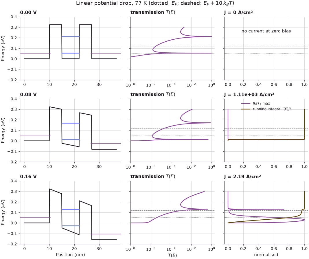
At zero bias the two Fermi levels coincide and no current flows, although the transmission has its sharp peak at C1. At 0.08 V the resonance has moved down into the occupied states of the emitter; the current spectrum is a single sharp line at the resonance and the running integral jumps from 0 to 1 there: practically all the current flows through C1. At 0.16 V C1 has dropped below the emitter band edge (here at $E=0$). The current is 500 times smaller and flows at low energies, through the off-resonant transmission (the tail of the C1 Lorentzian), with only a small step where C2, many $k_BT$ above the Fermi level, adds its share. Note also that under bias the transmission maximum stays below 1: the biased double barrier is no longer symmetric.

5. Resonance energies and widths against bias#

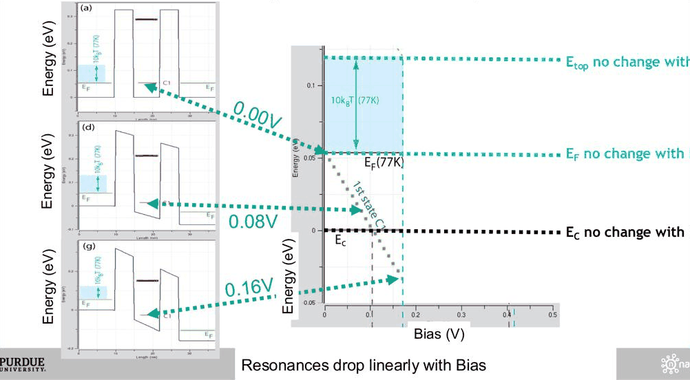
The lecture's slides 23–27 follow the resonance energies as the bias rises. With a linear drop the emitter band edge $E_c$, the Fermi level $E_F$ and the barrier top $E_{top}$ do not move (they are on the emitter side), while each resonance drops roughly linearly. The center of the well is halfway through the drop region, so a state localised in the center drops by about $qV/2$.

Slide 25: band diagrams at 0, 0.08 and 0.16 V and the first resonance energy against bias — Slide 25. Band diagrams at 0, 0.08 and 0.16 V (left) and the first resonance energy against bias (right). $E_c$, $E_F$ and $E_{top}$ do not change with bias; the resonance drops linearly.

Code18 lines · cell 19

VB = np.round(np.arange(0.0, 0.501, 0.02), 3)
En, Wn, hi = [], [], []  # C1, C2 energies and widths; higher states as (V, E, width)
for v in VB:
    r = nemo.resonances(rtd, potential=-v * ramp, emin=-v - 0.25, emax=0.45)
    order = np.argsort(r["energy"])
    e, g = r["energy"][order], r["width"][order]
    narrow = g < 0.05  # C1 and C2 are narrow; broad states above the barrier tops are shown as dots
    En.append(e[narrow][:2])
    Wn.append(g[narrow][:2])
    hi += [(v, ek, gk) for ek, gk in zip(e[~narrow], g[~narrow]) if gk < 0.15]
En, Wn, hi = np.array(En), np.array(Wn), np.array(hi)
for k in range(2):
    slope = np.polyfit(VB, En[:, k], 1)[0]
    print(
        f"C{k + 1}: dE/dV = {slope:.3f} eV/V;  width {1e3 * Wn[0, k]:.3g} meV at 0 V -> "
        f"{1e3 * Wn[-1, k]:.3g} meV at {VB[-1]:.1f} V"
    )
print(f"higher states: widths {1e3 * hi[:, 2].min():.0f}-{1e3 * hi[:, 2].max():.0f} meV")

C1: dE/dV = -0.538 eV/V;  width 0.0298 meV at 0 V -> 0.493 meV at 0.5 V
C2: dE/dV = -0.517 eV/V;  width 1.08 meV at 0 V -> 11.9 meV at 0.5 V
higher states: widths 53-105 meV

Code16 lines · cell 20

fig, (a1, a2) = plt.subplots(1, 2, figsize=(10, 3.8))
cols = style.sweep(2)
for k in range(2):
    a1.plot(VB, En[:, k], "o-", ms=3, color=cols[k], label=f"C{k + 1}")
    a2.semilogy(VB, 1e3 * Wn[:, k], "o-", ms=3, color=cols[k], label=f"C{k + 1}")
a1.plot(hi[:, 0], hi[:, 1], ".", color=style.CONTEXT, label="higher states")
a2.semilogy(hi[:, 0], 1e3 * hi[:, 2], ".", color=style.CONTEXT, label="higher states")
a1.axhline(0, color=style.REFERENCE, lw=1)
a1.text(0.005, 0.005, "$E_c$ (emitter)", va="bottom")
a1.axhspan(EF77, EF77 + 10 * kB * 77, color=style.CONTEXT, alpha=0.25, label="$E_F$ to $E_F+10k_BT$ (77 K)")
a1.axhline(EF300 + 10 * kB * 300, color=style.CONTEXT, ls="--", lw=1, label="$E_F+10k_BT$ (300 K)")
a1.set(xlabel="Bias (V)", ylabel="Energy (eV)", ylim=(-0.3, 0.45), title="Resonance energies")
a2.set(xlabel="Bias (V)", ylabel="Width $\\Gamma$ (meV)", title="Resonance widths")
a1.legend(fontsize=7, ncol=2)
a2.legend(fontsize=8)
fig.tight_layout();

The ground state falls at 0.538 eV per volt, close to the factor 1/2 expected for a state centred halfway through the drop; C2 falls at 0.517 eV/V. The two slopes are not equal, and the broad states above the barrier tops (grey dots) fall at still different rates and even cross each other, so the traces are not parallel; the lecture leaves the reason as a homework question (exercise 1 below). The widths grow with bias: C1 from 0.0298 meV at 0 V to 0.493 meV at 0.5 V, C2 from 1.08 meV to 11.9 meV. The bias lowers the effective height of the collector barrier seen by the state, so the electron escapes faster to the right.

The plot also shows the rule the lecture draws from slides 28–30. A current turn-on happens when a resonance comes down into the thermally excited sea of electrons, the band from $E_F$ to roughly $E_F + 10\,k_BT$; a turn-off happens when the resonance passes under the emitter conduction band edge $E_c$. The conduction band edge and the temperature define the energy window of the electron supply.

6. Current–voltage characteristics at 77 K and 300 K#

Integrating $J(E)$ at every bias gives the I–V curve. At 77 K the window is narrow (10 $k_BT$ = 66 meV) and the features are sharp; at 300 K it is 258 meV wide, so higher, broader resonances contribute already at low bias.

Code18 lines · cell 23

V = np.round(np.arange(0.0, 0.5001, 0.01), 3)
IV = {T: np.array([spectrum(v, T, n=1200)["J"] for v in V]) for T in (77, 300)}


def peaks(J):
    """First peak, the valley after it and the second peak of an N-shaped curve."""
    i1 = next(i for i in range(1, len(J) - 1) if J[i] >= J[i - 1] and J[i] > J[i + 1])
    i2 = i1 + int(np.argmin(J[i1 : i1 + 25]))
    i3 = i2 + int(np.argmax(J[i2:]))
    return i1, i2, i3


for T, J in IV.items():
    i1, i2, i3 = peaks(J)
    print(
        f"{T:3d} K: first peak {J[i1]:7.0f} A/cm^2 at {V[i1]:.2f} V, valley {J[i2]:7.1f} A/cm^2 at "
        f"{V[i2]:.2f} V (PVR {J[i1] / J[i2]:.0f}); second peak {J[i3]:7.0f} A/cm^2 at {V[i3]:.2f} V"
    )

 77 K: first peak    1144 A/cm^2 at 0.07 V, valley     1.8 A/cm^2 at 0.13 V (PVR 638); second peak    5538 A/cm^2 at 0.37 V
300 K: first peak    1182 A/cm^2 at 0.08 V, valley   469.4 A/cm^2 at 0.11 V (PVR 3); second peak    6174 A/cm^2 at 0.36 V

Code9 lines · cell 24

fig, (a1, a2) = plt.subplots(1, 2, figsize=(10, 3.8))
for T, c in ((77, style.OPEN_NEMO), (300, style.REFERENCE)):
    a1.plot(V, IV[T] / 1e3, color=c, lw=2, label=f"{T} K")
    a2.semilogy(V, IV[T], color=c, lw=2, label=f"{T} K")
a1.set(xlabel="Bias (V)", ylabel="Current density (kA/cm²)", title="I–V, linear scale")
a2.set(xlabel="Bias (V)", ylabel="Current density (A/cm²)", title="I–V, log scale")
a1.legend()
a2.legend()
fig.tight_layout();

Slide 30: resonance energies with the 10 kT windows at 77 K and 300 K, and the I–V curves at both temperatures — Slide 30. (a) Energies of the first four states against bias, with the 10 $k_BT$ windows at 77 K (blue) and 300 K (rose). (b) I–V characteristics at 300 K (thick) and 77 K (thin), linear scale. Dashed arrows mark the turn-on (blue) and turn-off (red) voltages read from (a).

The computed curves have the shape of the lecture's: a first peak at 0.07–0.08 V from C1, a deep valley at 77 K, and a large second peak near 0.37 V from C2. At 77 K the first peak is 1144 A/cm$^2$ and the valley 1.8 A/cm$^2$, a PVR of 638. At 300 K the first valley is filled in by the thermal tail through C2 and the PVR drops to 3, the typical value the lecture quotes. The magnitudes are about a factor of two below the slide (whose 300 K second peak is about $1.3\times10^4$ A/cm$^2$ against 6174 A/cm$^2$ here), which is within what different material parameters and contact models give: the lecture's tool uses its own masses, contact lengths and grid. The valley after the second peak is shallow: the turn-off of C2 leaves the broad upper states, which already reach into the supply window.

7. Which resonance carries the current?#

Broad resonances carry a lot of current even when they sit far up in the Boltzmann tail of the supply. To see this, the current spectrum at a given bias is split at the midpoints between neighbouring resonance energies and each part is assigned to the resonance it contains. The lecture quotes, at 300 K, about 75% of the current through C1 and 25% through C2 at the first peak (0.08 V), and 70% through C2 and 30% through C3 and C4 at the second peak (0.38 V).

Code16 lines · cell 28

def shares(v, T):
    s = spectrum(v, T)
    r = s["res"]
    keep = r["width"] < 0.15  # drop broad features that are not states of the well
    e = np.sort(r["energy"][keep])
    below = int(np.sum(e <= 0))  # resonances already under the emitter band edge
    e = e[e > 0]
    cuts = np.concatenate([[-np.inf], 0.5 * (e[1:] + e[:-1]), [np.inf]])
    dJ = np.concatenate([[0], 0.5 * (s["Je"][1:] + s["Je"][:-1]) * np.diff(s["E"])])
    out = [dJ[(s["E"] > a) & (s["E"] <= b)].sum() / s["J"] for a, b in zip(cuts[:-1], cuts[1:])]
    return {f"C{below + k + 1}": f for k, f in enumerate(out) if f > 0.005}


for v in (0.08, 0.38):
    sh = shares(v, 300)
    print(f"300 K, {v:.2f} V: " + ", ".join(f"{k} {100 * f:.0f}%" for k, f in sh.items()))

300 K, 0.08 V: C1 76%, C2 23%
300 K, 0.38 V: C2 89%, C3 9%, C4 1%

Slide 33: resonance widths and energies against bias on a log scale, with the current split at 0.08 V — Slide 33. Width (red) and energy (green) of the first three resonances against bias. C2 is about 40 times broader than C1, C3 about 40 times broader than C2. Inset (b): at 0.08 V and 300 K the normalised cumulative current (green) jumps by 75% at C1 and by 25% at C2.

At the first peak the split computed here, 76% through C1 and 23% through C2, is the lecture's. At 0.38 V C2 carries 89% and the upper states 10%, less than the lecture's 30%; the upper states of this device sit higher in energy. The mechanism is the width: the current carried by a narrow resonance is roughly proportional to its width times the supply at its energy, $\Gamma_n\,\ln(1+e^{(E_F-E_n)/k_BT})$. A resonance 40 times broader can be several $k_BT$ higher in energy and still carry a comparable current. This is why at room temperature the valley current in the turn-off region is carried by the higher, very broad resonances, and why a high PVR at room temperature is hard to reach.

8. Exploration: thicker or thinner barriers#

The barrier thickness sets the resonance widths exponentially, and with them the peak current. The cell below repeats the 77 K I–V calculation for 4, 5 and 6 nm barriers (the drop region is adjusted to each structure) and prints the C1 width, the first peak, the valley and the PVR.

Code14 lines · cell 32

fig, ax = plt.subplots(figsize=(6, 3.8))
VX = np.round(np.arange(0.0, 0.30001, 0.01), 3)
for b, c in zip((4.0, 5.0, 6.0), style.sweep(3)):
    dev = make_rtd(barrier=b)
    J = np.array([spectrum(v, 77, device=dev, n=800)["J"] for v in VX])
    i1, i2, _ = peaks(J)
    g1 = nemo.resonances(dev, emax=0.15)["width"][0]
    print(
        f"barrier {b:.0f} nm: C1 width {1e3 * g1:.3g} meV, peak {J[i1]:8.1f} A/cm^2 at {VX[i1]:.2f} V, "
        f"valley {J[i2]:6.2f} A/cm^2, PVR {J[i1] / J[i2]:.0f}"
    )
    ax.semilogy(VX, J, color=c, lw=2, label=f"{b:.0f} nm barriers")
ax.set(xlabel="Bias (V)", ylabel="Current density (A/cm²)", title="First peak at 77 K vs barrier thickness")
ax.legend();

barrier 4 nm: C1 width 0.149 meV, peak   5856.0 A/cm^2 at 0.07 V, valley  32.63 A/cm^2, PVR 179
barrier 5 nm: C1 width 0.0298 meV, peak   1141.8 A/cm^2 at 0.07 V, valley   1.79 A/cm^2, PVR 638
barrier 6 nm: C1 width 0.00595 meV, peak    223.1 A/cm^2 at 0.07 V, valley   0.10 A/cm^2, PVR 2332

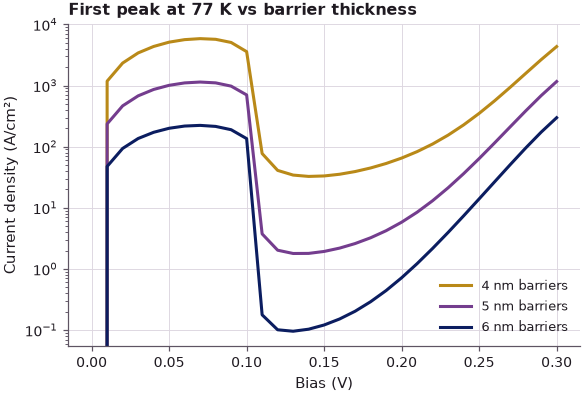
Each nanometre of AlGaAs changes the C1 width, and with it the peak current, by a factor of about five (0.149, 0.0298 and 0.00595 meV; 5856, 1142 and 223 A/cm$^2$). The valley current falls even faster, because it comes through C2, whose width also shrinks, so the PVR rises from 179 to 2332. High current and low valley pull in opposite directions; that trade-off is the design problem the PVR and the power window describe.

Summary#

An RTD is a double barrier between doped contacts. Its resonance is an energy bandpass filter that the bias pulls through the electron supply of the emitter: turn-on when the resonance enters the thermal sea (within about 10 $k_BT$ above $E_F$), turn-off when it passes under the emitter band edge. The result is an N-shaped I–V curve with negative differential resistance.
With a linear potential drop across barriers and well, the resonances drop almost linearly with bias, the ground state at about half the bias, the excited states with different slopes.
The current density is $J=\int J(E)\,dE$ with $J(E)$ the transmission times the supply difference; the running integral shows which resonances carry the current.
At 77 K the I–V features are sharper than at 300 K because the supply window is narrower.
Resonance widths grow by large factors from state to state, so the broad excited resonances carry a lot of current, at the first peak and especially in the valley at room temperature.
Figures of merit: peak-to-valley ratio (typically 3, a 1993 record of 87, applications want about 1000) and the power window $\Delta V\,\Delta I$.

Exercises#

The lecture's homework. Why are the resonance energy traces not parallel? Plot the probability density of C1 and C3 at 0.2 V (use the x0 and sigma returned by nemo.resonances, or the local density of states from nemo.Transport(...).solve(...)) and relate the slope $dE_n/dV$ to where each state sits in the linear drop. Hint: a state that extends over the whole drop region, or above the barriers, does not feel the potential of the well center only.
Change the temperature in the I–V calculation to 150 K and 200 K. At which temperature does the first valley disappear?
Use the shares function at 0.06, 0.08 and 0.10 V and at 77 K. How does the share of C2 change with temperature at the first peak?
Make the well 5 nm wide instead of 7 nm. Where are C1 and C2 now, and how does the I–V curve change?