Lecture 24.2

Long-range strain — expanding the strain domain

In the lecture

The numerical experiment: a dome-shaped dot, 30 nm in diameter and 5 nm high, embedded in GaAs whose buffer around the dot grows from 4 to 20 nm in every direction; the atoms have free outer surfaces, the electrons hard walls.
The electron ground state rises by about 175 meV for a pure InAs dot and 100 meV for an In${0.6}$Ga${0.4}$As dot as the buffer grows, as much as the dot's confining potential; the holes move by about 35 meV. Nothing has converged at 20 nm.
A reminder from Section 23: hydrostatic compression raises the conduction band and lowers the valence band; biaxial strain splits heavy and light holes.
"Classical" local band edges along lateral and vertical cuts show why: the strain inside and around the dot changes with the buffer, and the GaAs is strained tens of nanometres away.
Something is unphysical: with free surfaces the small dot expands the whole crystal. A substrate should be fixed to the GaAs lattice and the sides periodic.

In this notebook

You repeat the experiment with open-nemo's finite-element elasticity solver and an effective-mass model on the strained local band edges: the electron and hole ground states of the InAs and the In${0.6}$Ga${0.4}$As dome for buffers of 4–20 nm, the band shifts under hydrostatic and biaxial strain, the local band-edge profiles through the dot for a small and a large buffer, the vertical expansion of the free crystal, and the number of atoms the largest buffer means.

Run the notebookEvery number and figure on this page comes from it. Change it, rerun it, take it further.

Download .ipynb View on GitHub

Run it on your own machine

The notebook needs open-nemo (Python ≥ 3.10 and a C++20 compiler; BLAS/LAPACK).

git clone https://github.com/denphi/open-nemo.git && cd open-nemo
python3 -m venv .venv && source .venv/bin/activate
pip install -e ".[notebooks]"
jupyter lab From_Atoms_to_Devices/10_long_range_strain/24_2_expanding_the_strain_domain.ipynb

Code13 lines · cell 1

import time

import numpy as np
import matplotlib.pyplot as plt
import opennemo as nemo
from opennemo.models import kp
from opennemo.solvers import elasticity as el
from opennemo.solvers.poisson import Grid
from opennemo.structures.shapes import Box, Dome
from opennemo.visualization import style

style.use(notebook=True)
T_START = time.time()

1. Ground-state energies depend strongly on the buffer#

The dot of this section is a dome (half an ellipsoid of revolution) of 15 nm radius and 5 nm height, without a wetting layer, embedded in GaAs. The GaAs buffer around it is made larger and larger, the same thickness $b$ in all six directions, and both the strain and the electronic structure are recomputed on the whole domain. The outer surfaces are free for the atoms, so the crystal can expand in all three directions, and they are hard walls for the electrons.

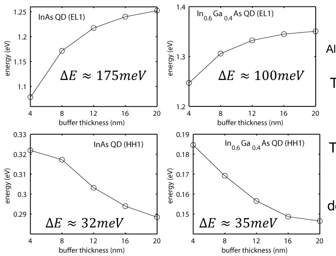Slide 5: electron and hole ground states against the buffer size Slide 5: ground-state energies of the pure InAs and the alloyed In$_{0.6}$Ga$_{0.4}$As dot as the GaAs buffer grows from 4 to 20 nm: the electrons rise by about 175 meV (InAs) and 100 meV (alloy), the holes change by about 32 and 35 meV.

The lecture's observations: the shift of the electron energy is huge, of the order of the dot's confining potential $\Delta E_c = E_c(\mathrm{GaAs}) - E_c(\mathrm{InGaAs})$; it is weaker for the alloyed dot, whose lattice constant is closer to that of GaAs; and the holes respond differently from the electrons, a sign that they feel different strain components.

We use the continuum model of Lecture 24.1: finite-element strain, local band edges from the strained 8-band k·p Hamiltonian at each point, and single-band effective-mass levels on them (electrons on $E_c$, holes on the top valence band with the heavy-hole masses). The material parameters are those of Vurgaftman et al. (2001) at 300 K, with In${0.6}$Ga${0.4}$As interpolated between InAs and GaAs.

Code25 lines · cell 3

GaAs = kp.material("GaAs", temperature=300)            # Vurgaftman et al. (2001), 300 K
InAs = kp.material("InAs", temperature=300)
E0 = GaAs.valence_band_offset                           # energy zero: unstrained GaAs valence-band top


def stiffness(m):
    """Cubic elastic stiffness (GPa, Voigt) of a k·p material."""
    return el.cubic_stiffness(m.c11, m.c12, m.c44)


def misfit(m):
    """Eigenstrain of m on the GaAs reference lattice: a_m / a_GaAs - 1."""
    return m.lattice_constant / GaAs.lattice_constant - 1


for m in (GaAs, InAs):
    print(f"{m.name}: a = {m.lattice_constant:.5f} nm, E_g = {m.band_gap:.3f} eV, "
          f"E_c = {m.valence_band_offset + m.band_gap - E0:+.3f} eV, "
          f"E_v = {m.valence_band_offset - E0:+.3f} eV, "
          f"a_c = {m.ac:+.2f} eV, m_e = {m.electron_mass:.3f} m0")
print(f"InAs misfit on GaAs: {100 * misfit(InAs):.2f} %")

InGaAs = kp.material("InGaAs", x=0.6, temperature=300)
print(f"{InGaAs.name}: a = {InGaAs.lattice_constant:.5f} nm, E_g = {InGaAs.band_gap:.3f} eV, "
      f"misfit on GaAs {100 * misfit(InGaAs):.2f} %")

GaAs: a = 0.56532 nm, E_g = 1.422 eV, E_c = +1.422 eV, E_v = +0.000 eV, a_c = -7.17 eV, m_e = 0.067 m0
InAs: a = 0.60583 nm, E_g = 0.354 eV, E_c = +0.564 eV, E_v = +0.210 eV, a_c = -5.08 eV, m_e = 0.026 m0
InAs misfit on GaAs: 7.16 %
InGaAs(x=0.6): a = 0.58963 nm, E_g = 0.667 eV, misfit on GaAs 4.30 %

Code44 lines · cell 4

VOIGT = [(0, 0), (1, 1), (2, 2), (1, 2), (0, 2), (0, 1)]
_LINEAR = {}


def local_edges(m, eps):
    """Local band edges (eV, from E0) of material m under the strains eps (n, 3, 3): the zone-centre
    eigenvalues of its 8-band k·p Hamiltonian (Bir-Pikus strain terms). Returns E_c, E_HH, E_LH; the
    heavy holes are the valence pair with the least |Z> character (z: growth axis)."""
    if m.name not in _LINEAR:                            # H(eps) = H0 + sum eps_ij D_ij: linear in eps
        h0 = kp.bulk_hamiltonian(m, np.zeros(3), 8)
        d = []
        for i, j in VOIGT:
            u = np.zeros((3, 3))
            u[i, j] = u[j, i] = 1.0
            d.append(kp.bulk_hamiltonian(m, np.zeros(3), 8, strain=u) - h0)
        _LINEAR[m.name] = h0, np.array(d)
    h0, d = _LINEAR[m.name]
    v = np.stack([eps[:, i, j] for i, j in VOIGT], -1)
    w, u = np.linalg.eigh(h0[None] + np.einsum("na,aij->nij", v, d))
    z = np.abs(u[:, 3, 2:6]) ** 2 + np.abs(u[:, 7, 2:6]) ** 2   # basis S, X, Y, Z per spin
    order = np.argsort(z, axis=1)
    top = w[:, 2:6]
    e_hh = np.take_along_axis(top, order[:, :2], 1).max(1)
    e_lh = np.take_along_axis(top, order[:, 2:], 1).max(1)
    return w[:, 6] - E0, e_hh - E0, e_lh - E0


def region_at(result, points):
    """Region index (0: the GaAs matrix, >0: the dot) of the finite-element cell containing each
    point: the cell whose material local_strain_at measures the strain against."""
    p = result.problem
    ids = []
    for d, a in enumerate(p.grid.axes):
        x = points[:, d]
        if p.periodic[d]:
            x = a[0] + np.mod(x - a[0], a[-1] - a[0])
        ids.append(np.clip(np.searchsorted(a, x, side="right") - 1, 0, len(a) - 2))
    return p.material[np.ravel_multi_index(tuple(ids), p.cell_shape)]


eps_test = np.array([[-0.05, 0.01, 0.0], [0.01, -0.05, 0.0], [0.0, 0.0, 0.04]])
direct = np.linalg.eigvalsh(kp.bulk_hamiltonian(InAs, np.zeros(3), 8, strain=eps_test)) - E0
print("direct 8-band:  E_c, top valence =", np.round(direct[[6, 5]], 5))
print("local_edges:    E_c, E_HH, E_LH  =", np.round(np.ravel(local_edges(InAs, eps_test[None])), 5))

direct 8-band:  E_c, top valence = [0.86859 0.32936]
local_edges:    E_c, E_HH, E_LH  = [0.86859 0.32936 0.1134 ]

Code69 lines · cell 5

HB2M = 0.0380998                                         # hbar^2 / 2 m0 (eV nm^2)


def bdd_hamiltonian(shape, h, inv_mass, potential):
    """Single-band BenDaniel-Duke operator -div (hbar^2 / 2m) grad + V on a box grid of spacings h
    (nm) with hard walls; inv_mass (n, 3): m0/m along x, y, z at each point."""
    import scipy.sparse as sp
    n = int(np.prod(shape))
    idx = np.arange(n).reshape(shape)
    diag = np.asarray(potential, dtype=float).copy()
    rows, cols, vals = [], [], []
    for ax in range(3):
        a = np.take(idx, range(shape[ax] - 1), axis=ax).ravel()
        b = np.take(idx, range(1, shape[ax]), axis=ax).ravel()
        t = HB2M * 0.5 * (inv_mass[a, ax] + inv_mass[b, ax]) / h[ax] ** 2
        rows += [a, b]
        cols += [b, a]
        vals += [-t, -t]
        np.add.at(diag, a, t)
        np.add.at(diag, b, t)
        for wall in (np.take(idx, [0], axis=ax).ravel(), np.take(idx, [shape[ax] - 1], axis=ax).ravel()):
            diag[wall] += HB2M * inv_mass[wall, ax] / h[ax] ** 2   # psi = 0 one step outside
    off = sp.coo_matrix((np.concatenate(vals), (np.concatenate(rows), np.concatenate(cols))), shape=(n, n))
    return off.tocsr() + sp.diags(diag)


def hole_inv_mass(m):
    """Heavy-hole m0/m in the plane (gamma1 + gamma2) and along z (gamma1 - 2 gamma2)."""
    return np.array([m.gamma1 + m.gamma2, m.gamma1 + m.gamma2, m.gamma1 - 2 * m.gamma2])


def dot_levels(result, dot, lo, hi, h=(1.0, 1.0, 0.5), num=1, holes=True):
    """Lowest electron and highest hole levels (eV, from E0) of a dot of material `dot` in GaAs, in
    the hard-wall box lo..hi (nm) on a grid of spacings h, with the strain and the regions of the
    finite-element `result`. Returns a dict with the levels, the grid and the band edges on it."""
    axes = [np.arange(lo[i] + h[i] / 2, hi[i], h[i]) for i in range(3)]
    shape = tuple(len(a) for a in axes)
    pts = np.stack(np.meshgrid(*axes, indexing="ij"), -1).reshape(-1, 3)
    ind = region_at(result, pts) > 0
    eps = result.local_strain_at(pts)
    ec, ev = np.empty(len(pts)), np.empty(len(pts))
    for m, sel in ((GaAs, ~ind), (dot, ind)):
        c, hh, lh = local_edges(m, eps[sel])
        ec[sel], ev[sel] = c, np.maximum(hh, lh)
    inv_me = 1.0 / np.where(ind, dot.electron_mass, GaAs.electron_mass)
    re = nemo.eigenstates(bdd_hamiltonian(shape, h, np.repeat(inv_me[:, None], 3, 1), ec), num=num)
    out = {"e": np.sort(re["energies"]), "e_states": re, "points": pts, "shape": shape, "axes": axes,
           "ec": ec, "ev": ev, "inside": ind}
    if holes:                                            # holes: lowest states of (kinetic - E_v)
        inv_mh = np.where(ind[:, None], hole_inv_mass(dot)[None], hole_inv_mass(GaAs)[None])
        rh = nemo.eigenstates(bdd_hamiltonian(shape, h, inv_mh, -ev), num=num)
        out["h"], out["h_states"] = -np.sort(rh["energies"]), rh
    return out


def graded_axis(lo, hi, core_lo, core_hi, h, h_max=2.0, growth=1.25):
    """Grid nodes from lo to hi (nm): spacing h on [core_lo, core_hi] around the dot, growing by
    `growth` per cell outside it up to h_max. Elasticity has no length scale, so the far buffer
    needs no fine grid."""
    def grow(start, end, sign):
        pts, x, s = [], start, h
        while True:
            s = min(s * growth, h_max)
            x += sign * s
            if (x >= end - 0.3 * s) if sign > 0 else (x <= end + 0.3 * s):
                return pts + [end]
            pts.append(x)
    core = list(np.arange(core_lo, core_hi + 1e-9, h))
    return np.array(grow(core_lo, lo, -1)[::-1] + core + grow(core_hi, hi, +1))

The finite-element grid is fine (1 nm laterally, 0.5 nm vertically) over the dot and grows geometrically up to 2 nm cells in the buffer, so a 20 nm buffer costs about a second. The strain is evaluated on the electronic grid, a box around the dot of the same spacings, with hard walls a distance $\min(b, 5\ \mathrm{nm})$ from the dot: Lecture 24.3 shows that the states do not reach further than that, and §2 of that notebook checks it for this model.

Code29 lines · cell 7

R, H = 15.0, 5.0
dome = Dome((0, 0, 0), (R, R, H))                                   # base at z = 0, apex at z = 5 nm
BUFFERS = [4, 8, 12, 16, 20]


def strain_free(m, b, fix_bottom=False):
    """Elastic equilibrium of the dome of material m in a GaAs box with buffer b (nm) on all six
    sides; free outer surfaces (rigid-body motion pinned), or the bottom face clamped."""
    xa = graded_axis(-R - b, R + b, -R - 1, R + 1, 1.0)
    za = graded_axis(-b, H + b, -1, H + 1, 0.5)
    prob = el.Elasticity.from_regions(Grid(xa, xa, za), [(None, stiffness(GaAs), 0.0),
                                                         (dome, stiffness(m), misfit(m))])
    if fix_bottom:
        prob.fix(np.isclose(prob.grid.nodes[:, 2], -b))
    return prob.solve()


strain, levels = {}, {}
t0 = time.time()
for m in (InAs, InGaAs):
    for b in BUFFERS:
        res = strain_free(m, b)
        e = min(b, 5.0)
        lv = dot_levels(res, m, (-R - e, -R - e, -e), (R + e, R + e, H + e))
        strain[m.name, b], levels[m.name, b] = res, lv
        i_c = np.argmin(np.linalg.norm(lv["points"] - [0, 0, 2.5], axis=1))
        print(f"{m.name:14s} buffer {b:2d} nm: e1 = {lv['e'][0]:.4f} eV, h1 = {lv['h'][0]:.4f} eV, "
              f"E_c at the dot's centre {lv['ec'][i_c]:.3f} eV")
print(f"{len(strain)} strain fields and {2 * len(levels)} levels in {time.time() - t0:.1f} s")

InAs           buffer  4 nm: e1 = 1.0460 eV, h1 = 0.2964 eV, E_c at the dot's centre 0.834 eV
InAs           buffer  8 nm: e1 = 1.1156 eV, h1 = 0.2861 eV, E_c at the dot's centre 0.913 eV
InAs           buffer 12 nm: e1 = 1.1471 eV, h1 = 0.2731 eV, E_c at the dot's centre 0.949 eV
InAs           buffer 16 nm: e1 = 1.1619 eV, h1 = 0.2654 eV, E_c at the dot's centre 0.965 eV
InAs           buffer 20 nm: e1 = 1.1695 eV, h1 = 0.2610 eV, E_c at the dot's centre 0.974 eV
InGaAs(x=0.6)  buffer  4 nm: e1 = 1.2437 eV, h1 = 0.2512 eV, E_c at the dot's centre 1.105 eV
InGaAs(x=0.6)  buffer  8 nm: e1 = 1.2944 eV, h1 = 0.2463 eV, E_c at the dot's centre 1.165 eV
InGaAs(x=0.6)  buffer 12 nm: e1 = 1.3163 eV, h1 = 0.2395 eV, E_c at the dot's centre 1.190 eV
InGaAs(x=0.6)  buffer 16 nm: e1 = 1.3263 eV, h1 = 0.2354 eV, E_c at the dot's centre 1.202 eV
InGaAs(x=0.6)  buffer 20 nm: e1 = 1.3313 eV, h1 = 0.2332 eV, E_c at the dot's centre 1.207 eV
10 strain fields and 20 levels in 17.5 s

Code14 lines · cell 8

fig, axes = plt.subplots(1, 2, figsize=(11, 3.8))
for k, m in enumerate((InAs, InGaAs)):
    e1 = np.array([levels[m.name, b]["e"][0] for b in BUFFERS])
    h1 = np.array([levels[m.name, b]["h"][0] for b in BUFFERS])
    axes[0].plot(BUFFERS, e1, marker="os"[k], **style.series(variant=k, label=m.name))
    axes[1].plot(BUFFERS, h1, marker="os"[k], **style.series(variant=k, label=m.name))
    print(f"{m.name:14s}: e1 rises by {1e3 * (e1[-1] - e1[0]):5.1f} meV, "
          f"h1 falls by {1e3 * (h1[0] - h1[-1]):4.1f} meV from b = 4 to 20 nm; the last step (16 -> 20 nm): "
          f"{1e3 * (e1[-1] - e1[-2]):+.1f} / {1e3 * (h1[-1] - h1[-2]):+.1f} meV")
axes[0].set(xlabel="GaAs buffer b (nm)", ylabel="electron ground state e1 (eV)", title="electrons")
axes[1].set(xlabel="GaAs buffer b (nm)", ylabel="hole ground state h1 (eV)", title="holes")
for ax in axes:
    ax.legend(frameon=False)
fig.tight_layout()

InAs          : e1 rises by 123.6 meV, h1 falls by 35.5 meV from b = 4 to 20 nm; the last step (16 -> 20 nm): +7.6 / -4.4 meV
InGaAs(x=0.6) : e1 rises by  87.6 meV, h1 falls by 18.1 meV from b = 4 to 20 nm; the last step (16 -> 20 nm): +5.0 / -2.3 meV

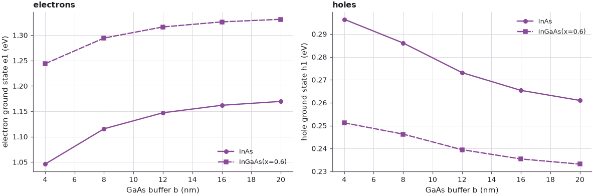
Figure computed by the notebook with open-nemo

The model reproduces the lecture's picture. As the buffer grows from 4 to 20 nm, the electron level of the InAs dot rises by about 120 meV (175 meV in the tight-binding calculation), that of the alloyed dot by about 90 meV (100 meV). The hole levels move much less, by 35 and 18 meV (32 and 35 meV on the slide). And none of the curves is flat at 20 nm: the last 4 nm still shift the InAs electron by 8 meV.

The absolute values are not the lecture's: the single-band model has no conduction-band non-parabolicity and its parameters are not the tight-binding ones. What both models share, and what matters here, is the dependence on the size of the strain domain.

2. A reminder: how strain moves the band edges#

Electrons and holes respond differently because they feel different parts of the strain.

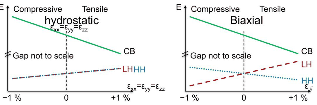Slide 6: band edges under biaxial and hydrostatic strain Slide 6: the conduction band and the heavy- and light-hole bands of GaAs or InAs under biaxial (left) and hydrostatic (right) strain, from −1 % (compression) to +1 % (tension).

Under hydrostatic strain $\varepsilon_{xx} = \varepsilon_{yy} = \varepsilon_{zz}$ the conduction band moves by $a_c \operatorname{tr}\varepsilon$: up under compression, down under tension. The valence bands move together by $a_v \operatorname{tr}\varepsilon$, down under compression. Biaxial strain (a layer squeezed in the plane and free to expand along $z$) also has a shear part that splits the heavy and the light holes by about $2|b|(\varepsilon_{zz} - \varepsilon_{xx})$. In a dot the strain is a three-dimensional mixture: the conduction band is the only clear indicator of compression or expansion, and the splitting of the valence bands the indicator of biaxial components.

Code18 lines · cell 10

e_scan = np.linspace(-0.01, 0.01, 41)
fig, axes = plt.subplots(1, 2, figsize=(11, 3.6), sharey=True)
for ax, kind in zip(axes, ("biaxial", "hydrostatic")):
    eps = np.zeros((len(e_scan), 3, 3))
    eps[:, 0, 0] = eps[:, 1, 1] = e_scan
    eps[:, 2, 2] = -2 * GaAs.c12 / GaAs.c11 * e_scan if kind == "biaxial" else e_scan
    ec, hh, lh = local_edges(GaAs, eps)
    gap = GaAs.band_gap
    for y, lab, col in ((ec - gap + 0.2, "$E_c$ (shifted down by $E_g$ − 0.2 eV)", style.sweep(3)[0]),
                        (hh, "$E_{HH}$", style.sweep(3)[1]), (lh, "$E_{LH}$", style.sweep(3)[2])):
        ax.plot(100 * e_scan, y, color=col, label=lab)
    ax.set(xlabel=f"in-plane strain ε_xx (%), {kind}", title=f"GaAs, {kind} strain")
    i = np.argmin(np.abs(e_scan + 0.01))
    print(f"{kind:11s} -1 %: dE_c = {1e3 * (ec[i] - gap):+6.1f} meV, dE_HH = {1e3 * hh[i]:+6.1f} meV, "
          f"dE_LH = {1e3 * lh[i]:+6.1f} meV")
axes[0].set_ylabel("band edge (eV)")
axes[0].legend(frameon=False, fontsize=8)
fig.tight_layout()

biaxial     -1 %: dE_c =  +76.9 meV, dE_HH =  +26.1 meV, dE_LH =  -41.5 meV
hydrostatic -1 %: dE_c = +215.1 meV, dE_HH =  -34.8 meV, dE_LH =  -34.8 meV

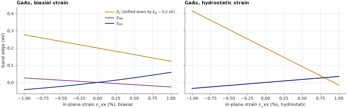
For GaAs, 1 % of hydrostatic compression raises the conduction band by about 215 meV and lowers both hole bands by 35 meV. 1 % of biaxial compression raises the conduction band by much less, 77 meV, because the expansion along $z$ undoes part of the volume change, and it splits the holes: the heavy hole moves up by 26 meV, the light hole down by 42 meV.

3. Local band edges through the dot#

What happens inside and around the dot as the buffer grows? The lecture answers with "classical" local band edges: walk along a line of As atoms, take each one's four neighbours, repeat that small cell periodically to make an infinite crystal, and compute its bulk band edges. The continuum analogue used here evaluates the 8-band k·p band edges of the local strain at each point of a line.

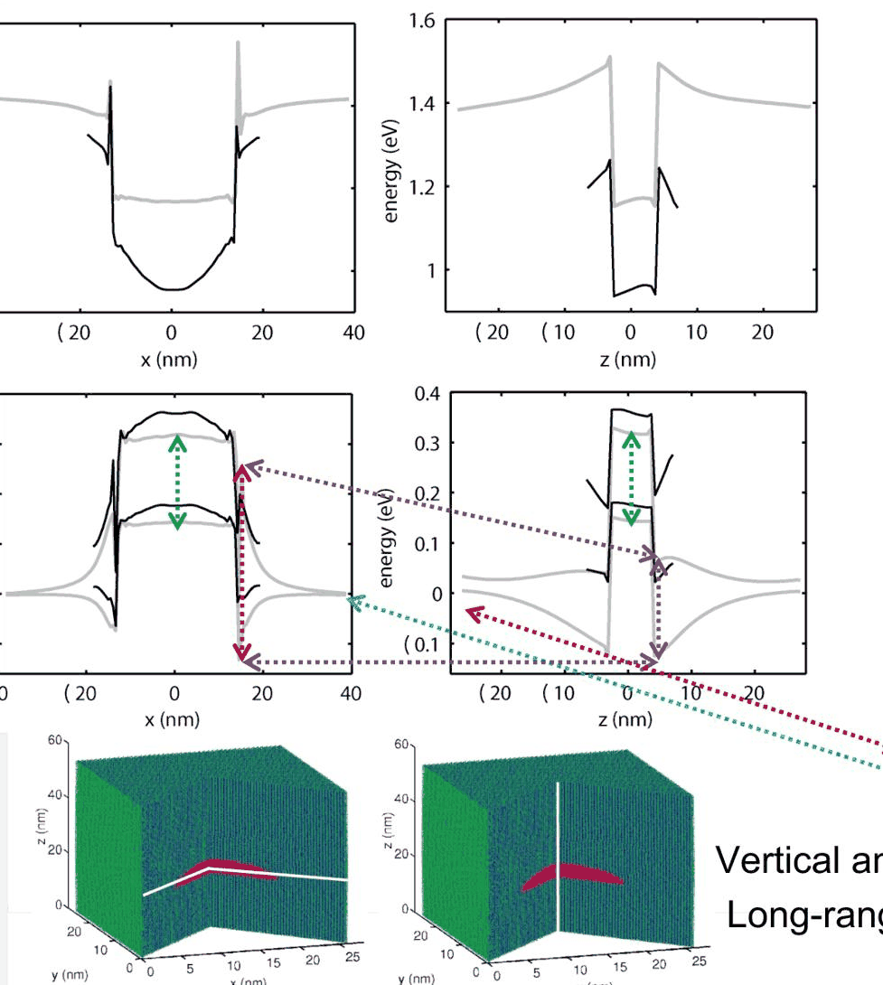Slide 12: local band edges along lateral and vertical cuts for two buffer sizes Slide 12: conduction-band edge (top) and heavy- and light-hole edges (bottom) along a lateral and a vertical cut through the InAs dot, for a small and a large buffer.

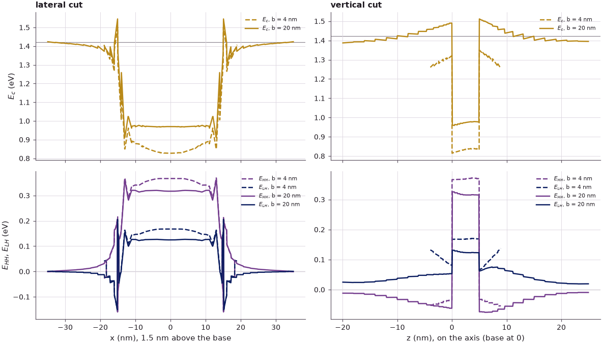
The cuts below go through the InAs dome of §1, laterally along $x$ at 1.5 nm above its base and vertically along its axis, for $b$ = 4 nm and $b$ = 20 nm.

Code33 lines · cell 12

def edges_along(res, m, pts):
    """E_c, E_HH, E_LH (eV) at the points: the dot material inside the dome, GaAs outside."""
    ind, eps = region_at(res, pts) > 0, res.local_strain_at(pts)
    out = np.empty((3, len(pts)))
    for mat, sel in ((GaAs, ~ind), (m, ind)):
        out[:, sel] = local_edges(mat, eps[sel])
    return out


Z_CUT = 1.5
cuts = {}
for b in (4, 20):
    s = np.linspace(-R - b + 0.05, R + b - 0.05, 701)
    t = np.linspace(-b + 0.05, H + b - 0.05, 501)
    cuts["lateral", b] = (s, edges_along(strain["InAs", b], InAs, np.c_[s, 0 * s, Z_CUT + 0 * s]))
    cuts["vertical", b] = (t, edges_along(strain["InAs", b], InAs, np.c_[0 * t, 0 * t, t]))

fig, axes = plt.subplots(2, 2, figsize=(11, 6.4), sharex="col")
for j, kind in enumerate(("lateral", "vertical")):
    for b, ls in ((4, "--"), (20, "-")):
        s, (ec, hh, lh) = cuts[kind, b]
        axes[0, j].plot(s, ec, ls=ls, color=style.sweep(3)[0], label=f"$E_c$, b = {b} nm")
        axes[1, j].plot(s, hh, ls=ls, color=style.sweep(3)[1], label=f"$E_{{HH}}$, b = {b} nm")
        axes[1, j].plot(s, lh, ls=ls, color=style.sweep(3)[2], label=f"$E_{{LH}}$, b = {b} nm")
    for i in range(2):
        axes[i, j].axhline((GaAs.band_gap, 0.0)[i], **style.series("context"))
    axes[1, j].set_xlabel(("x (nm), 1.5 nm above the base", "z (nm), on the axis (base at 0)")[j])
    axes[0, j].set_title(f"{kind} cut")
axes[0, 0].set_ylabel("$E_c$ (eV)")
axes[1, 0].set_ylabel("$E_{HH}$, $E_{LH}$ (eV)")
for ax in axes.ravel():
    ax.legend(frameon=False, fontsize=7)
fig.tight_layout()

Code16 lines · cell 13

def at(kind, b, x, band=0):
    s, e = cuts[kind, b]
    return e[band, np.argmin(np.abs(s - x))]


x_out = R * np.sqrt(1 - (Z_CUT / H) ** 2) + 0.5                      # GaAs, 0.5 nm beside the dot
print(f"E_c in the dot (x = 0): {at('lateral', 4, 0):.3f} eV (b = 4) -> "
      f"{at('lateral', 20, 0):.3f} eV (b = 20), "
      f"+{1e3 * (at('lateral', 20, 0) - at('lateral', 4, 0)):.0f} meV")
print(f"lateral GaAs, b = 20: E_c = {at('lateral', 20, x_out):.3f} eV beside the dot, "
      f"{at('lateral', 20, R + 19.9):.3f} eV at the outer surface (bulk {GaAs.band_gap:.3f})")
print(f"vertical GaAs, b = 20: E_c = {at('vertical', 20, H + 0.5):.3f} eV above the dot, "
      f"{at('vertical', 20, -0.5):.3f} eV below it, {at('vertical', 20, -19.9):.3f} eV at the bottom surface")
for kind, x in (("lateral", 0.0), ("lateral", x_out), ("vertical", H + 0.5), ("vertical", -19.9)):
    split = 1e3 * (at(kind, 20, x, 1) - at(kind, 20, x, 2))
    print(f"{kind:8s} x = {x:5.1f} nm, b = 20: E_HH - E_LH = {split:+5.0f} meV")

E_c in the dot (x = 0): 0.827 eV (b = 4) -> 0.970 eV (b = 20), +143 meV
lateral GaAs, b = 20: E_c = 1.305 eV beside the dot, 1.423 eV at the outer surface (bulk 1.422)
vertical GaAs, b = 20: E_c = 1.505 eV above the dot, 1.489 eV below it, 1.387 eV at the bottom surface
lateral  x =   0.0 nm, b = 20: E_HH - E_LH =  +192 meV
lateral  x =  14.8 nm, b = 20: E_HH - E_LH =  -188 meV
vertical x =   5.5 nm, b = 20: E_HH - E_LH =  -138 meV
vertical x = -19.9 nm, b = 20: E_HH - E_LH =   -37 meV

The local band edges make the long range of the strain visible:

In the dot, the conduction-band edge at the centre rises by about 140 meV between the two buffers, close to the shift of the electron level itself (the lecture: 175–220 meV). With the small buffer the surrounding GaAs is too thin to squeeze the InAs; the large buffer squeezes it harder.
Laterally, the GaAs right beside the dot is stretched ($E_c$ below the bulk 1.422 eV) and relaxes towards bulk at the outer surface, 20 nm away. Its holes are split by about 190 meV next to the dot, with the light hole on top: biaxial strain of the opposite sign from that in the dot, where the heavy hole lies 190 meV above the light hole (the lecture: about 380 and 170 meV).
Vertically, the GaAs above and below the dot is compressed ($E_c$ above 1.422 eV), but at the bottom surface of the box, 20 nm below the dot, it is expanded ($E_c$ = 1.39 eV), and its heavy and light holes are still almost 40 meV apart: the substrate is not relaxed.

4. Something is unphysical: the boundary conditions#

Slide 15: the setup of the numerical experiment and its boundary conditions 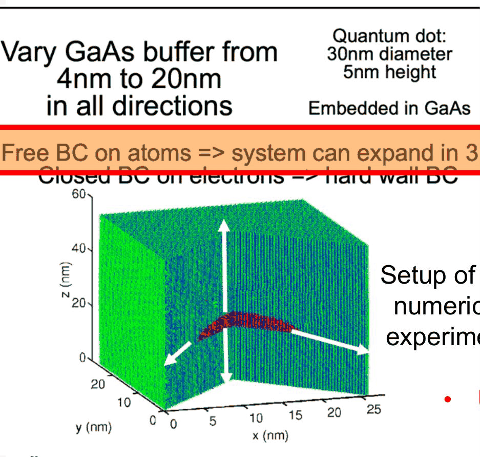Slide 15: what is wrong with the free-surface experiment: the small dot expands the whole crystal, and the substrate below it is stretched vertically instead of being GaAs. A substrate should be fixed to the GaAs lattice, the sides periodic, the top free (thin cap) or fixed (deeply buried dot).

A single dot grown on a GaAs wafer cannot stretch the wafer. With free outer surfaces, however, the crystal around the dot is a finite block, and the dot, 7 % larger than its cavity, pushes it apart. The vertical strain $\varepsilon_{zz}$ along the axis shows this for growing buffers, together with the same 20 nm block whose bottom face is clamped to the GaAs lattice, the way a substrate holds it.

Code31 lines · cell 15

t0 = time.time()
clamped = strain_free(InAs, 20, fix_bottom=True)
lv_c = dot_levels(clamped, InAs, (-R - 5, -R - 5, -5), (R + 5, R + 5, H + 5))
t_clamped = time.time() - t0

def bottom_report(res, b, label):
    z = np.linspace(-b + 0.05, H + b - 0.05, 400)
    eps = res.local_strain_at(np.c_[0 * z, 0 * z, z])
    tr = np.trace(eps, axis1=1, axis2=2)
    i = np.argmin(np.abs(z + b - 0.5))                                 # GaAs 0.5 nm above the bottom face
    ec = local_edges(GaAs, eps[i:i + 1])[0][0]
    print(f"{label:24s}: 0.5 nm above the bottom face eps_xx = {100 * eps[i, 0, 0]:+.2f} %, "
          f"eps_zz = {100 * eps[i, 2, 2]:+.2f} %, tr eps = {100 * tr[i]:+.2f} %, E_c = {ec:.3f} eV")
    return z, tr


fig, ax = plt.subplots(figsize=(7, 3.8))
for k, b in enumerate((4, 12, 20)):
    z, tr = bottom_report(strain["InAs", b], b, f"free, b = {b} nm")
    ax.plot(z, 100 * tr, color=style.sweep(4)[k], label=f"free, b = {b} nm")
z, tr = bottom_report(clamped, 20, "bottom clamped, b = 20 nm")
ax.plot(z, 100 * tr, color=style.sweep(4)[3], ls="--", label="bottom clamped, b = 20 nm")
ax.axvspan(0, H, color=style.CONTEXT, alpha=0.15, lw=0)
ax.axhline(0, **style.series("context"))
ax.set(xlabel="z (nm), on the dot's axis (dot: shaded)", ylabel="tr ε (%)", ylim=(-1.6, 2.4),
       title="volume change along the axis, InAs dot")
ax.legend(frameon=False, fontsize=8)
fig.tight_layout()
e_free = levels["InAs", 20]
print(f"b = 20 nm: e1 = {e_free['e'][0]:.4f} eV (free) vs {lv_c['e'][0]:.4f} eV (bottom clamped); "
      f"h1 = {e_free['h'][0]:.4f} vs {lv_c['h'][0]:.4f} eV ({t_clamped:.1f} s)")

free, b = 4 nm          : 0.5 nm above the bottom face eps_xx = +1.97 %, eps_zz = -1.86 %, tr eps = +2.09 %, E_c = 1.273 eV
free, b = 12 nm         : 0.5 nm above the bottom face eps_xx = +1.11 %, eps_zz = -1.01 %, tr eps = +1.20 %, E_c = 1.336 eV
free, b = 20 nm         : 0.5 nm above the bottom face eps_xx = +0.45 %, eps_zz = -0.42 %, tr eps = +0.48 %, E_c = 1.388 eV
bottom clamped, b = 20 nm: 0.5 nm above the bottom face eps_xx = +0.02 %, eps_zz = -0.16 %, tr eps = -0.11 %, E_c = 1.431 eV
b = 20 nm: e1 = 1.1695 eV (free) vs 1.1750 eV (bottom clamped); h1 = 0.2610 vs 0.2569 eV (2.0 s)

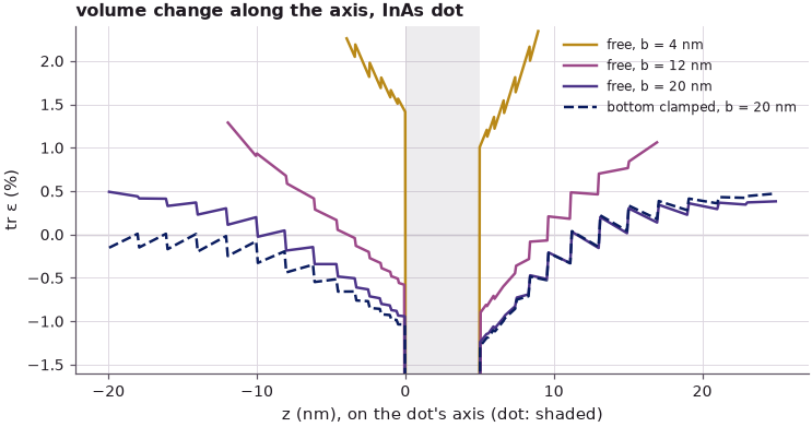
With free surfaces, the GaAs just above the bottom face is expanded: its volume grows by 2.1 % for the 4 nm buffer, 1.2 % for 12 nm and still 0.5 % for 20 nm, which lowers its $E_c$ by 149, 86 and 34 meV. The dot pushes the finite block apart sideways ($\varepsilon_{xx} > 0$), and the bottom of the block follows. Clamping the bottom face to the GaAs lattice removes this stretch ($\varepsilon_{xx}$ = 0.02 %), and leaves the substrate below the dot slightly compressed ($\operatorname{tr}\varepsilon = -0.11$ %, $E_c$ = 1.431 eV), as one expects. Here it moves the confined levels by only about 5 meV; the dot can still push the block's top and sides outward, which the bottom clamp alone does not prevent. Lecture 24.4 compares complete sets of boundary conditions.

The main conclusion of the lecture holds whatever the boundary: the strain is very far reaching, and a 20 nm buffer is not enough to converge it. How many atoms is that already? The domain of the largest buffer is 70 × 70 × 45 nm³:

Code6 lines · cell 17

a_gaas = 0.56532                                                     # nm
volume = (2 * R + 40) ** 2 * (H + 40)
cell = a_gaas**3
print(f"volume {volume:,.0f} nm^3, unit cell {cell:.8f} nm^3: {volume / cell / 1e6:.2f} million cells, "
      f"{8 * volume / cell / 1e6:.2f} million atoms")
print(f"notebook run time: {time.time() - T_START:.0f} s")

volume 220,500 nm^3, unit cell 0.18066875 nm^3: 1.22 million cells, 9.76 million atoms
notebook run time: 20 s

Almost ten million atoms, the size of a calculation on an early cluster around the year 2000, are not enough for strain convergence. The next lecture separates the two domains: a large one for the strain (atoms are cheap there) and a small one for the electrons.

Summary#

Growing the GaAs buffer around a 30 nm × 5 nm InAs dot from 4 to 20 nm raises its electron level by more than 100 meV (175 meV in the lecture's tight binding) and lowers the hole level by about 35 meV; for an In${0.6}$Ga${0.4}$As dot the electron shift is smaller. Nothing converges at 20 nm.
Electrons follow the hydrostatic strain through $a_c\operatorname{tr}\varepsilon$; the holes also feel the biaxial part that splits heavy and light holes, so the two carriers respond differently.
Local band edges along cuts through the dot show the strain changing in the dot and tens of nanometres into the GaAs, differently in the lateral and the vertical direction.
With free surfaces the dot expands the whole crystal: even the substrate 20 nm below it is stretched. Realistic boundary conditions fix the substrate and make the sides periodic.
The 20 nm buffer already holds 9.76 million atoms.

Exercises#

Extend the buffer sweep of §1 to 28 and 36 nm (the graded grid keeps the finite-element cost small). Does the InAs electron level converge, and how many atoms would that domain hold?
Repeat the sweep of §1 with the bottom face clamped (strain_free(m, b, fix_bottom=True)). Is the dependence on $b$ weaker?
In §3, plot $\operatorname{tr}\varepsilon$ and $\varepsilon_{zz} - \varepsilon_{xx}$ along the two cuts and check that $E_c$ follows the first and $E_{HH} - E_{LH}$ the second.