

Lecture 22.3
Optical matrix elements — an analytical expression for the dipole matrix element
In the lecture
- The dipole matrix element of the particle in a box in closed form, from the sine wave functions: finite when \(f - i\) is odd, zero when it is even.
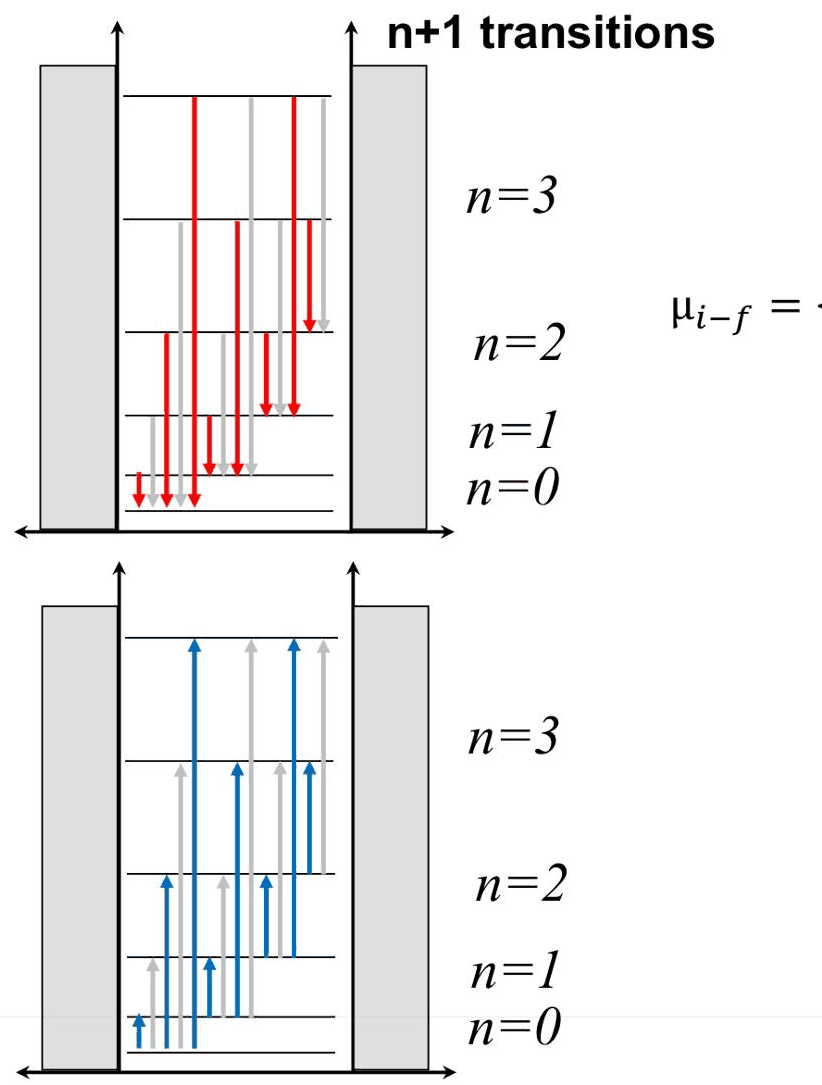
- Two limiting cases read off the formula: transitions between distant levels are weak (\(\mu \propto i/f^3\)), and the strength scales with the box size (\(\mu \propto L\)), so smaller structures couple more weakly at a given field.
- A summary of section 22: light couples states through the dipole matrix element, parity sets the selection rule, and the strength fades with the separation of the states and with the box size.
In this notebook
you derive the formula, compare it element by element with the dipole matrix elements of open-nemo's discretized box (and watch the discretization error vanish as the grid is refined), verify the \(i/f^3\) and nearest-neighbour limits, scale the box from 2 to 20 nm, and then use the library's oscillator strengths to see which quantities do and do not shrink with the box: the oscillator strength and its sum rule, and the spontaneous emission rate.
Run it on your own machine
The notebook needs open-nemo (Python ≥ 3.10 and a C++20 compiler; BLAS/LAPACK).
git clone https://github.com/denphi/open-nemo.git && cd open-nemo
python3 -m venv .venv && source .venv/bin/activate
pip install -e ".[notebooks]"
jupyter lab From_Atoms_to_Devices/08_optical_matrix_elements/22_3_analytical_dipole_matrix_element.ipynbCode
import numpy as np
import matplotlib.pyplot as plt
from matplotlib.ticker import NullFormatter, ScalarFormatter
from scipy.linalg import eigh_tridiagonal
import opennemo as nemo
from opennemo.core import units
from opennemo.simulations import optics
from opennemo.visualization import style

style.use(notebook=True)
1. The dipole matrix element of the box in closed form#
The lecture plugs the box states into the dipole integral. With the walls at \(x = \pm L/2\) and the states counted from \(n = 0\),
and the integral can be done by hand. Write \(p = i + 1\) and \(q = f + 1\) for the number of half-wavelengths of the two states (the sine's own quantum number), and shift the origin to the left wall: for \(i \ne f\) the shift adds \((L/2)\langle\psi_i|\psi_f\rangle = 0\), so it does not change the element. The product of sines becomes a difference of cosines, \(2\sin a\sin b = \cos(a - b) - \cos(a + b)\), and with \(\int_0^L x\cos(k\pi x/L)\,dx = (L/k\pi)^2\,[(-1)^k - 1]\) for an integer \(k \ne 0\),
Both brackets vanish when \(p - q\) is even, and both are \(-2\) when it is odd. Up to an overall sign, which depends on the phase convention of the states and drops out of every rate (\(\propto|\mu|^2\)), this is the slide's result:
One point of reading: in this formula \(i\) and \(f\) are the sine quantum numbers \(p, q = 1, 2, \dots\), not the labels \(n = 0, 1, \dots\) of the states; with the labels from zero, \(i = 0\) would make every element vanish. Since \(p - q = i - f\), the selection rule of lecture 22.2 is the same in both countings.
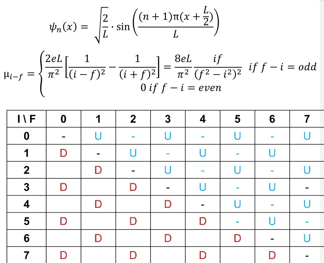
We check the formula against open-nemo. The effective-mass model (Heterostructure1D) of a 10 nm GaAs
layer with hard walls is a discretized box: the sines are exact on the grid points, but the energies
and the matrix elements carry a discretization error that should fall as the square of the grid
spacing \(\Delta\).
Code
M, L = 0.067, 10.0                     # GaAs electron mass (m0), box width (nm)
H2M0 = units.HBAR2_2M0
gaas = nemo.structures.materials.EffectiveMassMaterial("GaAs", M, 12.9)


def box(width=L, dx=0.02, num=8):
    """Hard-wall GaAs box exactly `width` nm wide (ψ = 0 one spacing beyond the end sites), centred:
    device, x (nm), lowest `num` energies (eV) and states ψ (1/√nm, columns)."""
    dev = nemo.Heterostructure1D([nemo.Layer(gaas, width - dx)], spacing=dx)
    x = dev.x - dev.x.mean()
    h = dev.hamiltonian.sparse.matrices[0].real
    e, psi = eigh_tridiagonal(h.diagonal(), h.diagonal(1), select="i", select_range=(0, num - 1))
    return dev, x, e, psi / np.sqrt(dx)


def dipoles(x, psi, dx):
    return np.abs(psi.T @ (x[:, None] * psi) * dx)     # |<ψi|x|ψf>| (nm)


def mu_analytic(n_i, n_f, width=L):
    """|<ψi|x|ψf>| (nm) of the box from the slide's formula; n_i, n_f are labels from 0."""
    p, q = np.asarray(n_i) + 1, np.asarray(n_f) + 1    # sine quantum numbers
    with np.errstate(divide="ignore", invalid="ignore"):
        val = 8 * width / np.pi**2 * p * q / (q**2 - p**2) ** 2
    return np.where((q - p) % 2 == 1, val, 0.0)


n = np.arange(8)
exact = mu_analytic(n[:, None], n[None, :])
dev, x, e, psi = box()
num = dipoles(x, psi, dev.spacing)
print("8eL/π² · if/(f² − i²)² in nm (upper triangle), |open-nemo| − formula in 1e-8 nm (lower triangle)")
print("     " + "".join(f"{f:9d}" for f in range(8)))
for i in range(8):
    row = []
    for f in range(8):
        row.append("        ·" if i == f else f"{exact[i, f]:9.4f}" if f > i
                   else f"{1e8 * (num[i, f] - exact[i, f]):9.2f}")
    print(f"{i:3d}  " + "".join(row))
8eL/π² · if/(f² − i²)² in nm (upper triangle), |open-nemo| − formula in 1e-8 nm (lower triangle)
             0        1        2        3        4        5        6        7
  0          ·   1.8013   0.0000   0.1441   0.0000   0.0397   0.0000   0.0163
  1      -0.01        ·   1.9454   0.0000   0.1838   0.0000   0.0560   0.0000
  2       0.00    -0.03        ·   1.9851   0.0000   0.2001   0.0000   0.0643
  3      -0.02     0.00    -0.06        ·   2.0014   0.0000   0.2084   0.0000
  4       0.00    -0.05     0.00    -0.11        ·   2.0097   0.0000   0.2132
  5      -0.03     0.00    -0.09     0.00    -0.16        ·   2.0144   0.0000
  6       0.00    -0.07     0.00    -0.15     0.00    -0.22        ·   2.0174
  7      -0.04     0.00    -0.13     0.00    -0.21     0.00    -0.29        ·
Code
allowed = exact > 0
print("  Δ (nm)   sites   largest relative error of the allowed elements   error / Δ⁴ (1/nm⁴)")
for dx in (0.1, 0.05, 0.025, 0.0125):
    d, xx, ee, pp = box(dx=dx)
    err = np.max(np.abs(dipoles(xx, pp, dx) - exact)[allowed] / exact[allowed])
    print(f"{dx:8.4f} {d.num_sites:7d}   {err:22.2e}{'':24s}{err / dx**4:8.3f}")
  Δ (nm)   sites   largest relative error of the allowed elements   error / Δ⁴ (1/nm⁴)
  0.1000      99                 1.62e-05                           0.162
  0.0500     199                 1.01e-06                           0.161
  0.0250     399                 6.29e-08                           0.161
  0.0125     799                 3.93e-09                           0.161
The formula and the open-nemo box agree to better than \(10^{-8}\) nm on the 0.02 nm grid, and the relative error falls by 16 each time the spacing halves (the last column is constant). The energies of the discretized box converge only as \(\Delta^2\), but its eigenvectors are the sines sampled exactly at the grid points, so what remains is the error of summing \(\psi_i\,x\,\psi_f\) on the grid instead of integrating it, and its \(\Delta^2\) term vanishes because the integrand and its slope are zero at the walls. Every forbidden element is zero in both.
2. Limiting cases: distant levels couple weakly#
The formula looks awkward, the lecturer admits, but its limits are telling. If the final state is far above the initial one, \(f \gg i\), then \(f^2 - i^2 \approx f^2\) and
large jumps, from a low to a very high quantum number or back down, are allowed by parity but weak. The strongest transitions are those between neighbours, where the first term of the bracket, \(1/(i - f)^2\), is largest. For neighbours \(f = i + 1\) the element tends to a constant,
Code
dev40, x40, e40, psi40 = box(dx=0.01, num=40)                # 40 states on a 0.01 nm grid
X40 = dipoles(x40, psi40, dev40.spacing)
f_all = np.arange(1, 40)

fig, axs = plt.subplots(1, 2, figsize=(11, 4.2))
ax = axs[0]
for i, c in zip((0, 1, 2, 4), style.sweep(4)):
    fs = f_all[(f_all > i) & ((f_all - i) % 2 == 1)]
    ax.loglog(fs + 1, X40[i, fs] / L, "o", ms=4, color=c, label=f"open-nemo, i = {i}")
    ax.loglog(fs + 1, mu_analytic(i, fs) / L, "-", lw=0.8, color=c)
    ax.loglog(fs + 1, 8 / np.pi**2 * (i + 1) / (fs + 1.0) ** 3, ":", lw=0.8, color=c)
ax.set(xlabel="sine quantum number of the final state, f + 1", ylabel="|⟨ψᵢ|x|ψ_f⟩| / L",
       title="allowed transitions from state i (dotted: 8i/π²f³)", xticks=[2, 3, 5, 10, 20, 40])
ax.xaxis.set_major_formatter(ScalarFormatter())
ax.xaxis.set_minor_formatter(NullFormatter())
ax.legend(fontsize=8, frameon=False)

ax = axs[1]
ii = np.arange(0, 39)
ax.plot(ii, X40[ii, ii + 1] / L, "o", ms=4, color=style.OPEN_NEMO, label="open-nemo, f = i + 1")
ax.plot(ii, mu_analytic(ii, ii + 1) / L, "-", lw=0.8, color=style.REFERENCE, label="formula")
ax.axhline(2 / np.pi**2, ls="--", color=style.CONTEXT, lw=1, label="2/π² (i → ∞)")
ax.set(xlabel="initial state i", ylabel="|⟨ψᵢ|x|ψᵢ₊₁⟩| / L", title="neighbouring levels")
ax.legend(fontsize=8, frameon=False)
fig.tight_layout()

print(f"|x_01| = {X40[0, 1]:.4f} nm, |x_03| = {X40[0, 3]:.4f} nm, |x_0,39| = {X40[0, 39]:.2e} nm")
print(f"|x_01| / |x_03| = {X40[0, 1] / X40[0, 3]:.1f}  (formula {mu_analytic(0, 1) / mu_analytic(0, 3):.1f})")
print(f"neighbours: |x_01| / L = {X40[0, 1] / L:.4f}, |x_38,39| / L = {X40[38, 39] / L:.4f}, "
      f"2/π² = {2 / np.pi**2:.4f}")
|x_01| = 1.8013 nm, |x_03| = 0.1441 nm, |x_0,39| = 1.27e-04 nm
|x_01| / |x_03| = 12.5  (formula 12.5)
neighbours: |x_01| / L = 0.1801, |x_38,39| / L = 0.2026, 2/π² = 0.2026
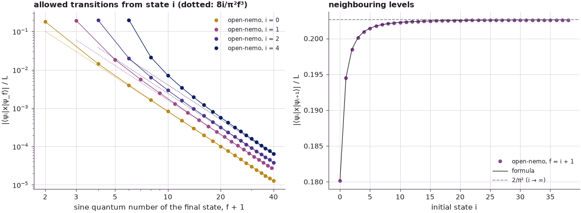
From the ground state the elements fall as \(1/f^3\): \(|x_{01}|\) is 12.5 times \(|x_{03}|\), and the jump from the ground state to the 40th level is four orders of magnitude weaker than the first. The far-jump asymptote \(8i/(\pi^2 f^3)\) (dotted) is approached from above for every initial state once \(f\) is a few times \(i\). Between neighbours the element grows slowly from \(0.180L\) and saturates at \(2L/\pi^2 = 0.203L\): in a box the strongest transitions are always the steps by one level.
3. Limiting case: small boxes couple weakly#
The second limit is the prefactor: every element is proportional to \(L\). The matrix element is a length, the size of the charge displacement that the light can drive between the two states, and a smaller box has less room for it. We compute \(|x_{01}|\) with open-nemo for boxes from 2 to 20 nm:
Code
widths = np.array([2, 3, 4, 5, 6, 8, 10, 12, 15, 20.0])
rows = []
for w in widths:
    d, xx, ee, pp = box(width=w, dx=0.01, num=40)
    tr = optics.transitions(d.hamiltonian.sparse.matrices[0], optics.velocity(d.hamiltonian),
                            (-1.0, -0.5), num_conduction=40, num_valence=0)
    fosc = optics.oscillator_strengths(tr["energies"], tr["matrix"][0])
    rows.append((dipoles(xx, pp, d.spacing)[0, 1], ee[1] - ee[0], fosc[0, 1], fosc[0, 1:].sum()))
x01, de01, f01, f_sum = map(np.array, zip(*rows))
print("  L (nm)  |x01| (nm)  |x01|/L   E1 - E0 (meV)   f01·m*/m0   Σf f0f·m*/m0 (40 states)")
for w, a, d_e, fo, fs in zip(widths, x01, de01, f01, f_sum):
    print(f"{w:7.1f} {a:10.4f} {a / w:9.4f} {1e3 * d_e:13.1f} {fo * M:12.4f} {fs * M:14.4f}")
print(f"16/(9π²) = {16 / (9 * np.pi**2):.4f};  analytic f01 m*/m0 = 256/(27π²) = {256 / (27 * np.pi**2):.4f}")
  L (nm)  |x01| (nm)  |x01|/L   E1 - E0 (meV)   f01·m*/m0   Σf f0f·m*/m0 (40 states)
    2.0     0.3603    0.1801        4208.9       0.9606         0.9999
    3.0     0.5404    0.1801        1870.7       0.9606         0.9999
    4.0     0.7205    0.1801        1052.3       0.9607         1.0000
    5.0     0.9006    0.1801         673.5       0.9607         1.0000
    6.0     1.0808    0.1801         467.7       0.9607         1.0000
    8.0     1.4410    0.1801         263.1       0.9607         1.0000
   10.0     1.8013    0.1801         168.4       0.9607         1.0000
   12.0     2.1615    0.1801         116.9       0.9607         1.0000
   15.0     2.7019    0.1801          74.8       0.9607         1.0000
   20.0     3.6025    0.1801          42.1       0.9607         1.0000
16/(9π²) = 0.1801;  analytic f01 m*/m0 = 256/(27π²) = 0.9607
\(|x_{01}|/L = 16/(9\pi^2) = 0.180\) for every width: the dipole matrix element is strictly proportional to the box size, as the lecture states. At a given optical field, a smaller box couples more weakly.
The same table shows that this is not the whole story, and this is the exploration of this notebook. The level spacing grows as \(1/L^2\) (from 42 meV at 20 nm to 4.2 eV at 2 nm, where the infinite-wall model has long stopped describing a real well). The oscillator strength combines the two,
and \(L^{-2}\cdot L^2\) makes it independent of the size: \(f_{01} = 256/(27\pi^2)\,m_0/m^* = 0.961\,m_0/m^*\)
for every box. The library's optics.oscillator_strengths, computed from the velocity operator, gives
exactly that, and the sum over all final states approaches the Thomas–Reiche–Kuhn sum rule
\(\sum_f f_{0f} = m_0/m^*\) (the 0 → 1 transition alone carries 96 % of it). Rates that weigh
\(|\mu|^2\) with powers of the transition frequency therefore do not shrink with the box. The spontaneous
emission rate of lecture 22.1, \(A \propto \omega^3|x|^2 \propto L^{-6}L^2\), even grows as \(L^{-4}\):
Code
n_r = 3.3                                              # refractive index of GaAs
omega = de01 / units.HBAR                              # rad/s
A = (n_r * units.Q**2 * omega**3 * (x01 * 1e-9) ** 2
     / (3 * np.pi * units.EPS0 * units.HBAR * units.Q * units.C_LIGHT**3))
slope = np.polyfit(np.log(widths), np.log(A), 1)[0]

fig, axs = plt.subplots(1, 3, figsize=(13, 3.8))
axs[0].plot(widths, x01, "o-", color=style.OPEN_NEMO, ms=4, label="open-nemo")
axs[0].plot(widths, 16 * widths / (9 * np.pi**2), "--", color=style.REFERENCE, lw=1, label="16L/9π²")
axs[0].set(xlabel="box width L (nm)", ylabel="|⟨ψ₀|x|ψ₁⟩| (nm)", title="dipole matrix element ∝ L")
axs[1].plot(widths, f01 * M, "o-", color=style.OPEN_NEMO, ms=4, label="f₀₁")
axs[1].plot(widths, f_sum * M, "s-", color=style.sweep(2)[0], ms=4, label="Σ_f f₀f (40 states)")
axs[1].axhline(256 / (27 * np.pi**2), ls="--", color=style.REFERENCE, lw=1, label="256/27π²")
axs[1].set(xlabel="box width L (nm)", ylabel="oscillator strength (m₀/m*)", ylim=(0.9, 1.02),
           title="oscillator strength: size independent")
axs[2].loglog(widths, A, "o-", color=style.OPEN_NEMO, ms=4)
axs[2].set(xlabel="box width L (nm)", ylabel="A₁₀ (1/s)", xticks=[2, 3, 5, 10, 20],
           title=f"spontaneous emission, fit ∝ L^({slope:.2f})")
axs[2].xaxis.set_major_formatter(ScalarFormatter())
axs[2].xaxis.set_minor_formatter(NullFormatter())
for ax in axs[:2]:
    ax.legend(fontsize=8, frameon=False)
fig.tight_layout()
print(f"A10: {A[0]:.2e} 1/s at {widths[0]:.0f} nm, {A[-1]:.2e} 1/s at {widths[-1]:.0f} nm; "
      f"power law L^{slope:.3f}")
A10: 1.21e+10 1/s at 2 nm, 1.21e+06 1/s at 20 nm; power law L^-4.000
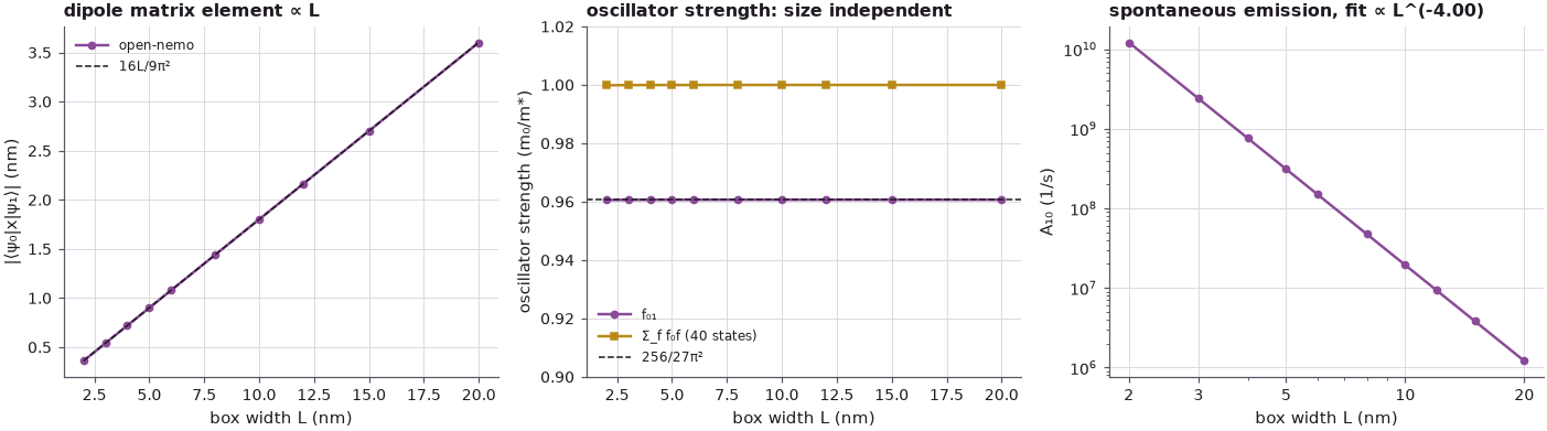
So "smaller dots give weaker optical coupling" is a statement about the matrix element itself, the coupling energy \(e\mathcal{E}|x_{if}|\) at a given field, which is what this section is about. The absorption strength per transition, measured by the oscillator strength, does not depend on the size, and the radiative rate grows steeply as the box shrinks, here as \(L^{-4}\) (the fit over 2–20 nm prints the exponent).
4. Summary of section 22#
The lecture closes the section with its summary, which the three notebooks have now computed:
- Light couples states through the dipole matrix element. The oscillating field adds \(H' = e\mathcal{E}_0\cos(\omega t)\,x\), which mixes the confined states; \(\mu_{if} = e\int\psi_i^*\,x\,\psi_f\,dx\) decides whether a transition happens, and the rate goes as \(|\mu_{if}|^2\) (lecture 22.1).
- Parity sets the selection rule. Even ↔ odd: the integrand is even, \(\mu \ne 0\), allowed (0 → 1, 1 → 2). Even ↔ even and odd ↔ odd: the integrand is odd, \(\mu = 0\), forbidden (0 → 2, 0 → 4, 1 → 3). A transition is allowed only when \(f - i\) is odd (lecture 22.2).
- The strength fades with the separation of the states and with the box size. \(\mu_{if} = \frac{8eL}{\pi^2}\frac{if}{(f^2-i^2)^2}\): neighbouring levels couple most strongly, and \(\mu \propto i/f^3\) far apart; \(\mu \propto L\), so smaller boxes give a weaker coupling at a given field (this notebook).
Summary#
- The dipole matrix element of the box is \(\frac{8eL}{\pi^2}\frac{if}{(f^2-i^2)^2}\) for \(f - i\) odd and zero otherwise, with \(i, f\) the sine quantum numbers (state label + 1); its sign is a phase convention.
- open-nemo's discretized box reproduces every element, with an error that falls as \(\Delta^4\) (below \(10^{-8}\) nm on a 0.02 nm grid).
- Far jumps are weak (\(\propto i/f^3\); ground state to level 40: four orders of magnitude below 0 → 1); neighbouring levels are strongest and saturate at \(2L/\pi^2\).
- \(|x_{01}| = 0.180\,L\) at every width, but the oscillator strength \(f_{01} = 0.961\,m_0/m^*\) is size independent (Thomas–Reiche–Kuhn sum \(m_0/m^*\)), and the spontaneous emission rate grows as \(L^{-4}\).
Exercises#
- Use
mu_analyticto show that \(\sum_f |\langle\psi_0|x|\psi_f\rangle|^2 = \langle\psi_0|x^2|\psi_0\rangle\) (closure; the diagonal term vanishes because \(\langle x\rangle = 0\) in the centred box) and evaluate \(\langle x^2\rangle\) numerically frompsi. - Replace the infinite box by a finite GaAs well in 0.25 eV barriers (layers of an
EffectiveMassMaterialwithconduction_band_edge=0.25, as in lecture 22.2) and compute \(|x_{01}|\) for widths from 3 to 20 nm. Where does it depart from \(0.180L\), and why does it not keep shrinking? - Compute the oscillator strengths \(f_{0f}\) for \(f = 1, 3, 5\) from the formula
(\(f_{0f} = \frac{2m^*}{\hbar^2}(E_f - E_0)|x_{0f}|^2\) in units of \(m_0/m^*\)) and compare with
optics.oscillator_strengths. - For the 1 → 2 transition (labels from 0), find how \(A_{21}\) scales with \(L\) and compare its value with that of 0 → 1 at \(L = 10\) nm.
Further reading#
- Lecture 22.1: the dipole matrix element and Lecture 22.2: allowed and forbidden transitions.
- Optical transitions and absorption of quantum wells: the intersubband oscillator strength of a real GaAs/AlGaAs well against the infinite-well 0.961, and full absorption spectra.
- Excitons in quantum wells and wires: how the Coulomb attraction redistributes the oscillator strength of interband transitions.
- GaAs momentum matrix elements: where the intra-atomic dipole sits.
- L. C. West and S. J. Eglash, "First observation of an extremely large-dipole infrared transition within the conduction band of a GaAs quantum well", Appl. Phys. Lett. 46, 1156 (1985): the intersubband dipole of a real well.
- D. J. Griffiths, Introduction to Quantum Mechanics (Cambridge University Press): the infinite square well and the Thomas–Reiche–Kuhn sum rule.