Lecture 21.4

NEMO 3-D — eigenvalues: Lanczos

Lecture page Video Slides

In the lecture

The size of the problem: a dot of 50 million atoms with 20 orbitals each gives a Hamiltonian of order \(10^9\), whose dense storage would take some 16,000 PB.
Stored sparsely it is "only" tens of GB, and a Lanczos solver never needs \(H\) itself, only products \(H\mathbf{q}\).
The Lanczos idea: a few thousand products build a small tridiagonal matrix \(T_k\) whose eigenvalues approach those of \(H\) — extreme eigenvalues first.
The wanted states lie in the middle of the spectrum, near the band gap; NEMO 3-D runs the recurrence as an open-ended loop until they emerge.
The Lanczos vectors form an orthonormal basis \(Q_k\); the factorization \(HQ_k = Q_kT_k + \mathbf{f}_k\mathbf{e}_k^T\) gives Ritz values, Ritz vectors and a free error estimate.
Eigenvectors without storing \(Q_k\): a second sweep regenerates the Lanczos vectors.

In this notebook

Redo the storage estimates of the slides.
Write the Lanczos recurrence of slide 6 in a few lines of numpy, apply it to the tight-binding Hamiltonian of a small GaAs nanocrystal built with open-nemo, and watch the Ritz values converge: extremes first, gap states last, with spurious copies from the lost orthogonality.
Compute eigenvectors with the second sweep and check the residual formula \(\|H\mathbf{x}-\lambda\mathbf{x}\| = \|\mathbf{f}_k\|\,|y_k|\).
Compare with open-nemo's NEMO 3-D-style solver lanczos_window_eigenstates.

Run the notebookEvery number and figure on this page comes from it. Change it, rerun it, take it further.

Download .ipynb View on GitHub

Run it on your own machine

The notebook needs open-nemo (Python ≥ 3.10 and a C++20 compiler; BLAS/LAPACK).

git clone https://github.com/denphi/open-nemo.git && cd open-nemo
python3 -m venv .venv && source .venv/bin/activate
pip install -e ".[notebooks]"
jupyter lab From_Atoms_to_Devices/07_quantum_dots_and_nemo3d/21_4_lanczos_eigenvalues.ipynb

Code10 lines · cell 1

import time
import numpy as np
import matplotlib.pyplot as plt
import opennemo as nemo
from opennemo.visualization import style
from opennemo.structures.structure import cluster
from opennemo.structures.shapes import Sphere
from opennemo.solvers.eigen import lanczos_window_eigenstates

style.use(notebook=True)

1. How large is the problem?#

A realistic dot involves millions of atoms: \(N \approx 50\) million atoms with a block of \(B = 20\) orbitals (sp3d5s* with spin) gives a Hamiltonian of size \((NB)^2\), i.e. \(NB = 10^9\) rows. Stored dense in double-precision complex numbers (16 bytes each) it would need

S = 10^9 \times 10^9 \times 16\ \text{bytes} \approx 2\times10^{4}\ \text{PB}

(the slides compare this with the storage of the largest internet companies, an infrastructure of hundreds of millions of dollars). It is also too much information: that is the size of the full eigenvector space, and nobody wants all \(10^9\) eigenvectors — only a few states in the middle of the spectrum, near the band gap. Stored sparsely, with only the diagonal block and the four neighbour blocks of each atom, the matrix shrinks enormously; and Lanczos never needs \(H\) itself, only its product with a vector, which can be recomputed on the fly (lecture 21.5).

Code9 lines · cell 3

N, B = 50e6, 20
dense = (N * B)**2 * 16
slide_sparse = N * B * 5 * 16                         # the slide's count: N x B x n(=5 blocks) x 16 bytes
nnz_row = 41                                          # measured for sp3d5s* + spin in lecture 21.3
every_nnz = N * B * nnz_row * (16 + 8)                # value + column index for every non-zero
print(f"dense storage:              {dense / 1e15:,.0f} PB")
print(f"sparse, slide's estimate:   {slide_sparse / 1e9:,.0f} GB")
print(f"sparse, every non-zero (CSR, 41 per row): {every_nnz / 1e12:.1f} TB")
print(f"three Lanczos vectors:      {3 * N * B * 16 / 1e9:,.0f} GB")

dense storage:              16,000 PB
sparse, slide's estimate:   80 GB
sparse, every non-zero (CSR, 41 per row): 1.0 TB
three Lanczos vectors:      48 GB

The slide's 80 GB counts one 16-byte number per row and neighbour block; storing every non-zero of the sp3d5s* matrix with its column index takes about 1 TB. Either way the matrix must be spread over many processors, while the Lanczos recurrence itself only needs three vectors of 16 GB each.

2. The Lanczos idea#

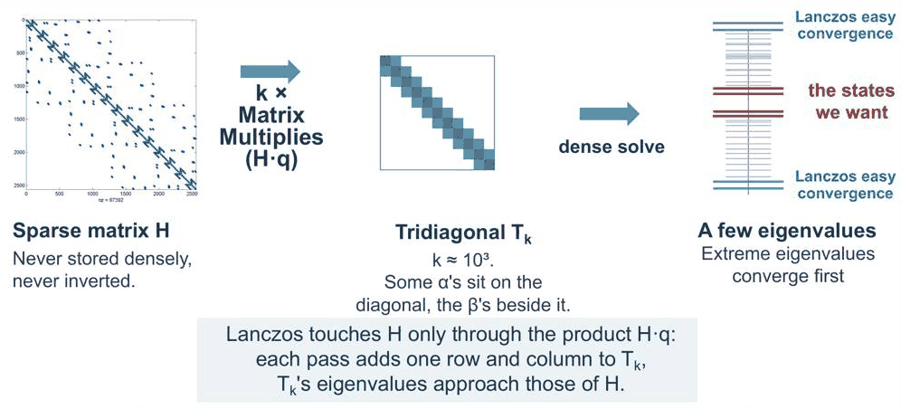
Slide 5: trade a 10^9 matrix for a 10^3 one — Slide 5: a sparse \(H\) of order \(10^9\), never stored densely nor inverted, is touched only through products \(H\mathbf{q}\); \(k \approx 10^3\) products build a tridiagonal \(T_k\) whose dense eigenvalues approximate those of \(H\). Extreme eigenvalues converge first; the states we want lie in the middle.

Starting from a random unit vector \(\mathbf{q}_1\), each step applies \(H\) once, projects the result on the current vector, subtracts the components along the last two vectors, and normalizes (slide 6):

\mathbf{w}_j = H\mathbf{q}_j,\qquad \alpha_j = \mathbf{q}_j^\dagger\mathbf{w}_j,\qquad \mathbf{f}_j = \mathbf{w}_j - \alpha_j\mathbf{q}_j - \beta_{j-1}\mathbf{q}_{j-1},\qquad \beta_j = \|\mathbf{f}_j\|,\qquad \mathbf{q}_{j+1} = \mathbf{f}_j/\beta_j .

Only the numbers \(\alpha_j\) (the projection of \(H\mathbf{q}_j\) on \(\mathbf{q}_j\)) and \(\beta_j\) (the norm of the residual) are kept. They form the tridiagonal matrix

T_k = \begin{pmatrix}\alpha_1 & \beta_1 & & \\ \beta_1 & \alpha_2 & \ddots & \\ & \ddots & \ddots & \beta_{k-1} \\ & & \beta_{k-1} & \alpha_k\end{pmatrix}.

The test object is the sp3d5s* Hamiltonian (no spin) of a GaAs nanocrystal of 2.6 nm diameter, passivated at the surface, small enough to be diagonalized densely for comparison.

Code14 lines · cell 5

GAAS = nemo.structures.materials.load("klimeck2002_sp3d5s")["GaAs"]
lat = nemo.structures.lattice.from_material(GAAS)
dot = cluster(lat, Sphere([0.05, 0.07, 0.03], 1.3))
H = nemo.models.tb.SlaterKoster(GAAS, passivation=30.0).build(dot).at(np.zeros(3)).tocsr()
n = H.shape[0]
t0 = time.perf_counter()
exact = np.linalg.eigvalsh(H.toarray())
print(f"{dot.num_atoms} atoms, H of order {n} with {H.nnz} non-zeros; "
      f"dense eigvalsh {time.perf_counter() - t0:.1f} s")
gap_lo = exact[exact < 0.8].max()                     # highest occupied level near the GaAs valence band
gap_hi = exact[exact > 0.8].min()                     # lowest empty level
print(f"spectrum {exact[0]:.2f} to {exact[-1]:.2f} eV (passivated levels near 30 eV); "
      f"gap states: HOMO {gap_lo:.4f} eV, LUMO {gap_hi:.4f} eV")
print(f"mean level spacing {(exact[-1] - exact[0]) / n * 1000:.1f} meV")

399 atoms, H of order 3990 with 142202 non-zeros; dense eigvalsh 6.8 s
spectrum -12.07 to 37.62 eV (passivated levels near 30 eV); gap states: HOMO -0.4179 eV, LUMO 2.3452 eV
mean level spacing 12.5 meV

Code25 lines · cell 6

def lanczos(H, k, seed=0):
    # plain Lanczos of slide 6, no reorthogonalization: returns alpha, beta (and the start vector)
    rng = np.random.default_rng(seed)
    q = rng.standard_normal(H.shape[0]) + 0j
    q /= np.linalg.norm(q)
    q0 = q.copy()
    q_prev, b_prev = np.zeros_like(q), 0.0
    alpha, beta = np.zeros(k), np.zeros(k)
    for j in range(k):
        w = H @ q
        alpha[j] = np.vdot(q, w).real
        f = w - alpha[j] * q - b_prev * q_prev
        beta[j] = np.linalg.norm(f)
        q_prev, q, b_prev = q, f / beta[j], beta[j]
    return alpha, beta, q0


K = 1500
t0 = time.perf_counter()
alpha, beta, q_start = lanczos(H, K)
print(f"{K} Lanczos steps in {time.perf_counter() - t0:.2f} s ({K} products H q)")


def ritz(k):
    return np.linalg.eigvalsh(np.diag(alpha[:k]) + np.diag(beta[:k - 1], 1) + np.diag(beta[:k - 1], -1))

1500 Lanczos steps in 0.16 s (1500 products H q)

Code21 lines · cell 7

steps = np.arange(20, K + 1, 20)
fig, (a1, a2) = plt.subplots(1, 2, figsize=(11, 4.4))
for k in steps:
    t = ritz(k)
    a1.plot(np.full(t.size, k), t, ",", color=style.OPEN_NEMO)
a1.set(xlabel="Lanczos steps k", ylabel="Ritz values (eV)", title="eigenvalues of T_k", ylim=(-14, 16))
a1.axhspan(gap_lo, gap_hi, color=style.CONTEXT, alpha=0.25, lw=0)
targets = {"lowest level": exact[0], "HOMO": gap_lo, "LUMO": gap_hi}
err = {name: [] for name in targets}
for k in steps:
    t = ritz(k)
    for name, e in targets.items():
        err[name].append(np.min(np.abs(t - e)))
for (name, e), c in zip(err.items(), style.sweep(3)):
    a2.semilogy(steps, np.maximum(e, 1e-15), color=c, label=name)
a2.set(xlabel="Lanczos steps k", ylabel="|nearest Ritz value − exact| (eV)", title="convergence")
a2.legend(frameon=False, fontsize=8)
fig.tight_layout()
for name in targets:
    conv = steps[np.argmax(np.array(err[name]) < 1e-8)] if min(err[name]) < 1e-8 else None
    print(f"{name:12s} {targets[name]:9.4f} eV: converged to 1e-8 eV after {conv} steps")

lowest level  -12.0680 eV: converged to 1e-8 eV after 80 steps
HOMO           -0.4179 eV: converged to 1e-8 eV after 580 steps
LUMO            2.3452 eV: converged to 1e-8 eV after 480 steps

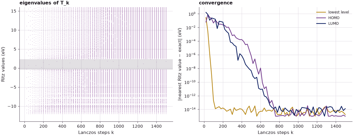
Figure computed by the notebook with open-nemo

The picture is the one of slide 5. The lowest eigenvalue, at the edge of the spectrum, converges to \(10^{-8}\) eV in 80 steps; the HOMO and LUMO, which lie in the middle of a spectrum about 50 eV wide (from \(-12.1\) to \(37.6\) eV, the top part being the passivation levels near 30 eV) where the levels are on average 12.5 meV apart, need 580 and 480 steps. Ordinary Lanczos codes stop after the extreme eigenvalues; NEMO 3-D instead keeps the loop open, monitors the Ritz values in the band gap, and peels out the gap states when they have converged.

The recurrence is run without reorthogonalization, so the computed vectors lose their orthogonality as soon as an eigenvalue converges, and converged eigenvalues reappear as copies ("ghosts") in \(T_k\). Counting the Ritz values that agree with the lowest eigenvalue shows it:

Code5 lines · cell 9

for k in (100, 500, 1000, 1500):
    t = ritz(k)
    print(f"k = {k:4d}: copies of the lowest eigenvalue in T_k: {np.sum(np.abs(t - exact[0]) < 1e-6)}, "
          f"Ritz values inside the gap ({gap_lo:.3f}, {gap_hi:.3f}) eV, strictly between: "
          f"{np.sum((t > gap_lo + 1e-4) & (t < gap_hi - 1e-4))}")

k =  100: copies of the lowest eigenvalue in T_k: 1, Ritz values inside the gap (-0.418, 2.345) eV, strictly between: 0
k =  500: copies of the lowest eigenvalue in T_k: 3, Ritz values inside the gap (-0.418, 2.345) eV, strictly between: 0
k = 1000: copies of the lowest eigenvalue in T_k: 7, Ritz values inside the gap (-0.418, 2.345) eV, strictly between: 1
k = 1500: copies of the lowest eigenvalue in T_k: 11, Ritz values inside the gap (-0.418, 2.345) eV, strictly between: 1

Copies multiply with the number of steps; they are harmless (they are exact eigenvalues, only repeated) and are removed by the test of Cullum and Willoughby that open-nemo's solver applies: a simple eigenvalue of \(T_k\) that is also an eigenvalue of \(T_k\) with its first row and column removed is spurious. Values strictly inside the gap that appear and disappear while converging are also discarded by that test and by the convergence check.

3. The Lanczos basis and the factorization#

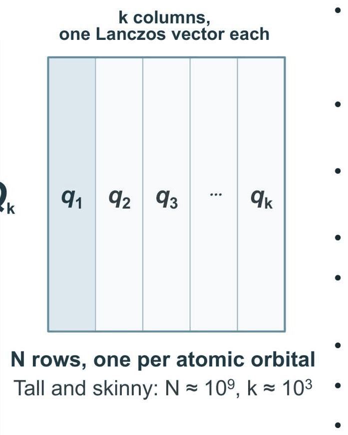
Slide 7: the Lanczos basis Q_k — Slide 7: the \(k\) Lanczos vectors are the columns of \(Q_k\), tall (\(N \approx 10^9\) rows) and thin (\(k \approx 10^3\) columns).

The vectors \(\mathbf{q}_1 \dots \mathbf{q}_k\) are orthonormal (in exact arithmetic) and span the Krylov space \(\{\mathbf{q}_1, H\mathbf{q}_1, H^2\mathbf{q}_1, \dots\}\). In this basis \(H\) becomes \(T_k = Q_k^\dagger H Q_k\), and the recurrence reads, as one matrix equation (slide 9),

HQ_k = Q_kT_k + \mathbf{f}_k\mathbf{e}_k^T ,

where \(\mathbf{e}_k\) is the last unit vector: \(H\) acting on the Lanczos vectors is tridiagonal apart from one leftover direction \(\mathbf{f}_k\). If \(T_k\mathbf{y} = \lambda\mathbf{y}\), then \(\lambda\) is a Ritz value (an estimate of an eigenvalue of \(H\)) and \(\mathbf{x} = Q_k\mathbf{y} = \sum_j y_j\mathbf{q}_j\) a Ritz vector, and multiplying the factorization by \(\mathbf{y}\) gives the error for free:

H\mathbf{x} - \lambda\mathbf{x} = (\mathbf{e}_k^T\mathbf{y})\,\mathbf{f}_k ,\qquad \|H\mathbf{x} - \lambda\mathbf{x}\| = \|\mathbf{f}_k\|\,|y_k| = \beta_k\,|y_k| .

The convergence of an eigenvalue can thus be monitored from \(T_k\) alone, without any vector. Storing all \(N \times k\) entries of \(Q_k\) is exactly what NEMO 3-D avoids: since the recurrence is deterministic, a second sweep from the same start vector regenerates the \(\mathbf{q}_j\) one by one and accumulates \(\mathbf{x} = \sum_j y_j\mathbf{q}_j\) on the fly, at the price of a second set of \(k\) products.

Code24 lines · cell 11

def second_sweep(H, q, k, Y):
    # regenerate q_1..q_k from the same start and accumulate x = sum_j y_j q_j for each column of Y
    X = np.zeros((H.shape[0], Y.shape[1]), complex)
    q_prev, b_prev = np.zeros_like(q), 0.0
    for j in range(k):
        X += np.outer(q, Y[j])
        w = H @ q
        f = w - alpha[j] * q - b_prev * q_prev
        q_prev, q, b_prev = q, f / beta[j], beta[j]
    return X


k = 1000
Tk = np.diag(alpha[:k]) + np.diag(beta[:k - 1], 1) + np.diag(beta[:k - 1], -1)
theta, Y = np.linalg.eigh(Tk)
pick = [np.argmin(np.abs(theta - e)) for e in (exact[0], gap_lo, gap_hi)]
X = second_sweep(H, q_start, k, Y[:, pick])
for i, name in zip(range(3), ("lowest", "HOMO", "LUMO")):
    x = X[:, i]
    lam = theta[pick[i]]
    true_res = np.linalg.norm(H @ x - lam * x) / np.linalg.norm(x)
    print(f"{name:7s} Ritz value {lam:9.5f} eV (exact {[exact[0], gap_lo, gap_hi][i]:9.5f}), "
          f"beta_k |y_k| = {beta[k - 1] * abs(Y[-1, pick[i]]):.1e}, ||Hx - lx||/||x|| = {true_res:.1e}, "
          f"||x|| = {np.linalg.norm(x):.3f}")

lowest  Ritz value -12.06802 eV (exact -12.06802), beta_k |y_k| = 2.2e-18, ||Hx - lx||/||x|| = 3.3e-14, ||x|| = 1.000
HOMO    Ritz value  -0.41791 eV (exact  -0.41791), beta_k |y_k| = 1.0e-11, ||Hx - lx||/||x|| = 1.0e-11, ||x|| = 1.000
LUMO    Ritz value   2.34517 eV (exact   2.34517), beta_k |y_k| = 6.6e-11, ||Hx - lx||/||x|| = 6.6e-11, ||x|| = 1.000

The free estimate \(\beta_k|y_k|\) and the residual of the vector built by the second sweep agree for the converged states, to round-off, and \(\|\mathbf{x}\| = 1.000\) for all three. (Because the computed \(\mathbf{q}_j\) are not exactly orthogonal, the norm need not be 1 in general; the solver normalizes the vectors at the end.) Where the estimate is not yet small, the eigenvalue has not converged and the vector is a mixture.

4. The NEMO 3-D solver in open-nemo#

lanczos_window_eigenstates implements this algorithm as NEMO 3-D did (Klimeck et al. 2002, §III F): the recurrence without reorthogonalization, Ritz values in an energy window checked every 200 steps with their error bounds, the Cullum–Willoughby test against spurious values, an open-ended loop with a minimum number of steps, and the second pass for the eigenvectors.

Code8 lines · cell 13

t0 = time.perf_counter()
res = lanczos_window_eigenstates(H, (gap_lo - 0.3, gap_hi + 0.3), tol=1e-8, min_steps=1000)
dt = time.perf_counter() - t0
inwin = exact[(exact > gap_lo - 0.3) & (exact < gap_hi + 0.3)]
print(f"window ({gap_lo - 0.3:.3f}, {gap_hi + 0.3:.3f}) eV: {res.attrs['steps']} steps, {dt:.1f} s")
print("Lanczos:", np.round(np.sort(res["energies"]), 5))
print("dense:  ", np.round(np.unique(np.round(inwin, 5)), 5))
print("residuals ||Hx - lx||:", np.array2string(np.asarray(res.attrs["residuals"]), precision=1))

window (-0.718, 2.645) eV: 2000 steps, 0.7 s
Lanczos: [-0.70355 -0.64727 -0.6384  -0.63399 -0.62896 -0.60608 -0.59849 -0.57235
 -0.4544  -0.43997 -0.41791  2.34517  2.44501  2.44796  2.45545  2.45664
  2.47278  2.48138  2.48318  2.56643  2.58118  2.58475  2.58739  2.62476
  2.63284  2.64015]
dense:   [-0.70355 -0.64727 -0.6384  -0.63399 -0.62896 -0.60608 -0.59849 -0.57235
 -0.4544  -0.43997 -0.41791  2.34517  2.44501  2.44796  2.45545  2.45664
  2.47278  2.48138  2.48318  2.56643  2.58118  2.58475  2.58739  2.62476
  2.63284  2.64015]
residuals ||Hx - lx||: [1.7e-10 5.6e-09 1.7e-10 7.7e-11 6.3e-09 2.5e-10 1.6e-11 2.2e-10 2.9e-10
 3.1e-10 7.4e-12 9.2e-09 1.4e-11 1.1e-11 2.9e-10 1.3e-10 8.4e-10 2.1e-10
 1.5e-09 5.2e-09 2.0e-09 2.6e-09 2.0e-09 4.8e-09 1.2e-09 6.4e-09]

The solver returns the distinct eigenvalues of the window, the gap states of the nanocrystal, with residuals between \(10^{-11}\) and \(10^{-8}\) eV, and all 26 match the dense diagonalization. This off-centre sphere has no degenerate levels in the window. Had it any (a nanocrystal centred on an atom has threefold levels from its cubic symmetry), they would be returned once: a single Lanczos recurrence only sees the start vector's component in each eigenspace, and nothing in \(\alpha\) and \(\beta\) distinguishes a degenerate eigenvalue from a simple one; open-nemo's block option runs several recurrences at once to recover the multiplicities.

The scaling argument of the lecture is now concrete: each step costs one sparse product, linear in the number of atoms; the memory is three vectors plus the \(\alpha\)'s and \(\beta\)'s; and the number of steps, \(10^3\)–\(10^4\) for gap states, depends on how wide the spectrum is and how close the wanted states are to their neighbours, not directly on the size of the matrix.

Summary#

An sp3d5s* Hamiltonian of 50 million atoms has order \(10^9\): about 16,000 PB dense, 80 GB to 1 TB sparse, and Lanczos needs only products \(H\mathbf{q}\) and three vectors.
The Lanczos recurrence keeps only \(\alpha_j\) and \(\beta_j\); the eigenvalues of the tridiagonal \(T_k\) converge to those of \(H\), extremes first. The gap states of a GaAs nanocrystal need about 500 steps; the lowest level needs 80.
Without reorthogonalization converged eigenvalues reappear as copies, removed by the Cullum–Willoughby test.
\(HQ_k = Q_kT_k + \mathbf{f}_k\mathbf{e}_k^T\) gives Ritz pairs and the residual \(\beta_k|y_k|\) for free; a second sweep builds the eigenvectors without storing \(Q_k\).
open-nemo's lanczos_window_eigenstates reproduces the NEMO 3-D solver and agrees with dense diagonalization.

Exercises#

Start the recurrence from a different random vector (seed=1). Do the convergence curves and the number of ghost copies change?
Add full reorthogonalization to lanczos (store the vectors and orthogonalize each new one against all previous ones). How do the ghosts and the convergence of the HOMO change, and what does it cost in memory for \(10^9\) rows?
Shift the spectrum: run Lanczos on \((H - \sigma)^2\) with \(\sigma\) in the gap ("folded spectrum", lecture 21.5). The gap states are now the lowest eigenvalues; how many products does their convergence take, counting two per step?