Lecture 21.6

NEMO 3-D — validation: does it work?

Lecture page Video Slides

In the lecture

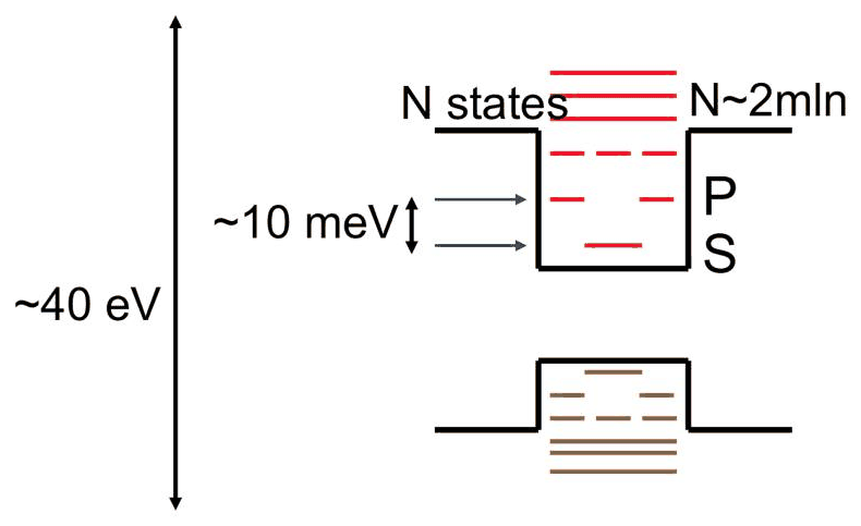
The wanted states of a quantum dot, the ground state and the first excited states, are some 10 meV apart, in a spectrum about 40 eV wide with millions of states: they are interior eigenvalues.
A first test of the Lanczos solver: the same dot computed in domains of 0.3, 6.7 and 21 million atoms (lateral sizes from 11.3 to 101.7 nm) gives the same ground and excited states, with the right symmetry.
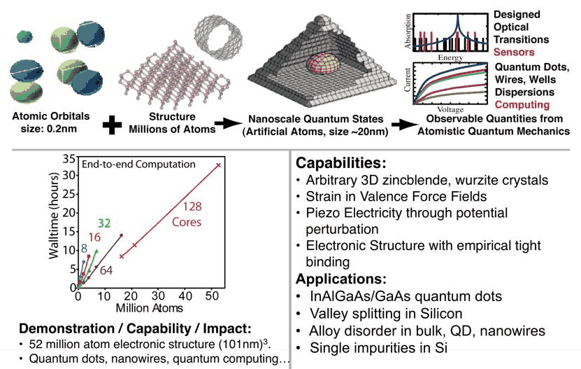
NEMO 3-D's capabilities: 52 million atoms, \((101\ \text{nm})^3\), computed end to end; zincblende and wurtzite crystals, valence force field strain, piezoelectric potentials, empirical tight binding.
Applications discussed in the following lectures: InAlGaAs/GaAs dots, valley splitting in silicon, alloy disorder, single impurities in silicon.

In this notebook

Estimate how far inside the spectrum the dot states of an InAs dot in GaAs lie.
Repeat the test of slide 3 with open-nemo: one InAs pyramid in GaAs boxes of four sizes, from 20,480 to 118,976 atoms, and compare the energies and wavefunctions of the lowest electron states.

Run the notebookEvery number and figure on this page comes from it. Change it, rerun it, take it further.

Download .ipynb View on GitHub

Run it on your own machine

The notebook needs open-nemo (Python ≥ 3.10 and a C++20 compiler; BLAS/LAPACK).

git clone https://github.com/denphi/open-nemo.git && cd open-nemo
python3 -m venv .venv && source .venv/bin/activate
pip install -e ".[notebooks]"
jupyter lab From_Atoms_to_Devices/07_quantum_dots_and_nemo3d/21_6_validation.ipynb

Code9 lines · cell 1

import time
import numpy as np
import matplotlib.pyplot as plt
import opennemo as nemo
from opennemo.visualization import style
from opennemo.structures.structure import Structure
from opennemo.solvers.eigen import lanczos_window_eigenstates

style.use(notebook=True)

1. Interior eigenstates#

Slide 2: a few dot states inside a spectrum of millions — Slide 2: the electron states S and P of a dot, about 10 meV apart, inside a band of \(N\) states (\(N \approx 2\) million) and a total spectrum about 40 eV wide.

The dot below is an InAs square pyramid, base 8 nm and height 3.5 nm, in GaAs, in the sp3s* basis (5 orbitals per atom). To keep the test about the eigensolver, the atoms sit on the ideal GaAs lattice: no relaxation and no strain (lectures 21.1–21.2 add them). The box is periodic, so the dot also sees its periodic images; the largest box has 26 × 26 × 22 cubic cells.

Code59 lines · cell 3

mats = nemo.structures.materials.load("klimeck2002_sp3s")
GAAS, INAS = mats["GaAs"], mats["InAs"]
lat = nemo.structures.lattice.from_material(GAAS)
a = GAAS.lattice_constant
DOT = nemo.structures.materials.alloy(GAAS, INAS)
BASE, HEIGHT = 8.0, 3.5


def dot_in_box(nxy, nz):
    # GaAs box of nxy x nxy x nz cubic cells with an InAs pyramid in its centre (ideal positions)
    cell, basis, sub = lat.conventional, lat.conventional_basis, lat.conventional_sublattice
    g = np.stack(np.meshgrid(np.arange(nxy), np.arange(nxy), np.arange(nz), indexing="ij"), -1).reshape(-1, 3)
    X = ((g @ cell)[:, None, :] + basis[None]).reshape(-1, 3)
    sublat = np.tile(sub, len(g))
    species = np.array([lat.species[i] for i in sublat], dtype=object)
    c0 = np.array([nxy * a / 2, nxy * a / 2, nz * a / 2 - HEIGHT / 2])     # centre of the base
    zr = X[:, 2] - c0[2]
    half = BASE / 2 * (1 - zr / HEIGHT)
    inside = ((zr >= 0) & (zr <= HEIGHT)
              & (np.abs(X[:, 0] - c0[0]) <= half) & (np.abs(X[:, 1] - c0[1]) <= half))
    species[inside & (species == "Ga")] = "In"
    s = Structure(X, list(species), np.diag([nxy * a, nxy * a, nz * a]), sublat, lat)
    return s, c0


def hamiltonian(s):
    # unrelaxed In-As bonds are 7 % shorter than InAs's own: widen the bond window to accept them
    return nemo.models.tb.SlaterKoster(DOT, spin=False, bond_tolerance=0.15).build(s).at(np.zeros(3))


s, c0 = dot_in_box(16, 10)
H = hamiltonian(s)


def spectrum_edges(H, k=300, seed=0):
    # the extreme Ritz values of a short Lanczos run converge first (lecture 21.4)
    q = np.random.default_rng(seed).standard_normal(H.shape[0]) + 0j
    q /= np.linalg.norm(q)
    q_prev, b_prev, al, be = np.zeros_like(q), 0.0, [], []
    for _ in range(k):
        w = H @ q
        al.append(np.vdot(q, w).real)
        f = w - al[-1] * q - b_prev * q_prev
        be.append(np.linalg.norm(f))
        q_prev, q, b_prev = q, f / be[-1], be[-1]
    t = np.linalg.eigvalsh(np.diag(al) + np.diag(be[:-1], 1) + np.diag(be[:-1], -1))
    return t[0], t[-1]


lo, hi = spectrum_edges(H)
e_bulk = np.linalg.eigvalsh(nemo.models.tb.SlaterKoster(GAAS).build(nemo.structures.structure.bulk(lat))
                            .dense(np.zeros(3)))
ec_gaas = e_bulk[e_bulk > 0.5].min()
print(f"smallest box: {s.num_atoms} atoms, H of order {H.shape[0]}, "
      f"spectrum {lo:.2f} to {hi:.2f} eV ({hi - lo:.1f} eV wide)")
print(f"mean level spacing {(hi - lo) / H.shape[0] * 1e3:.2f} meV; "
      f"GaAs conduction-band edge of this model {ec_gaas:.4f} eV")
print(f"valence states (4 of the 10 per Ga-As pair) below the dot states: {2 * s.num_atoms} "
      f"of {H.shape[0]}; above: {H.shape[0] - 2 * s.num_atoms}")

smallest box: 20480 atoms, H of order 102400, spectrum -13.00 to 12.75 eV (25.8 eV wide)
mean level spacing 0.25 meV; GaAs conduction-band edge of this model 1.4173 eV
valence states (4 of the 10 per Ga-As pair) below the dot states: 40960 of 102400; above: 61440

The spectrum of even the smallest box is about 26 eV wide in the sp3s* basis, from −13.0 to 12.75 eV (sp3d5s* adds higher levels and reaches the 40 eV of the slide), with on average one level every 0.25 meV. The dot's electron states lie inside it, just below the GaAs conduction-band edge: 40,960 of the 102,400 states lie below them and 61,440 above: this is why the Lanczos solver of lecture 21.4 runs until the interior Ritz values converge instead of stopping at the extremes.

2. The same dot in larger domains#

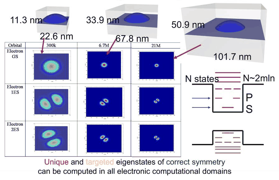
Slide 3: the same states in domains of 0.3, 6.7 and 21 million atoms — Slide 3: a lens-shaped dot on a wetting layer in domains of increasing size (lateral 11.3 to 101.7 nm); the ground state and the first two excited states have the same shape and symmetry in all of them.

We now put the same pyramid into four boxes, from 16 × 16 × 10 to 26 × 26 × 22 cubic cells, and ask the open-nemo Lanczos solver for the levels between 0.5 eV and 1.40 eV, i.e. below the GaAs conduction-band edge.

Code18 lines · cell 5

boxes = [(16, 10), (19, 14), (22, 18), (26, 22)]
results = []
for nxy, nz in boxes:
    t0 = time.perf_counter()
    s, c0 = dot_in_box(nxy, nz)
    H = hamiltonian(s)
    res = lanczos_window_eigenstates(H, (0.5, 1.40), tol=1e-8, count=3)
    dt = time.perf_counter() - t0
    order = np.argsort(res["energies"])
    E, V = np.asarray(res["energies"])[order], np.asarray(res["vectors"])[:, order]
    rho = (np.abs(V)**2).reshape(s.num_atoms, 5, -1).sum(1)          # probability per atom
    on_in = np.array(s.species) == "In"
    results.append(dict(n=(nxy, nz), atoms=s.num_atoms, X=np.asarray(s.positions) - c0, E=E, rho=rho,
                        w_in=rho[on_in].sum(0), steps=res.attrs["steps"], time=dt))
    print(f"{nxy:2d} x {nxy:2d} x {nz:2d} cells ({nxy * a:5.2f} x {nxy * a:5.2f} x {nz * a:5.2f} nm), "
          f"{s.num_atoms:6d} atoms: {res.attrs['steps']:4d} steps, {dt:5.1f} s; levels "
          + ", ".join(f"{e:.4f}" for e in E) + " eV; weight on In "
          + ", ".join(f"{w:.2f}" for w in rho[on_in].sum(0)))

16 x 16 x 10 cells ( 9.07 x  9.07 x  5.67 nm),  20480 atoms: 1400 steps,   4.3 s; levels 1.0746, 1.3055, 1.3071 eV; weight on In 0.41, 0.40, 0.40
19 x 19 x 14 cells (10.77 x 10.77 x  7.93 nm),  40432 atoms: 1400 steps,   8.4 s; levels 1.1051, 1.2986, 1.3001 eV; weight on In 0.42, 0.38, 0.38
22 x 22 x 18 cells (12.47 x 12.47 x 10.20 nm),  69696 atoms: 1600 steps,  15.9 s; levels 1.1144, 1.2940, 1.2955 eV; weight on In 0.44, 0.36, 0.36
26 x 26 x 22 cells (14.73 x 14.73 x 12.47 nm), 118976 atoms: 2000 steps,  31.8 s; levels 1.1175, 1.2904, 1.2918 eV; weight on In 0.45, 0.35, 0.35

Code19 lines · cell 6

nst = min(len(r["E"]) for r in results)
fig, axes = plt.subplots(nst, len(results), figsize=(3 * len(results), 3 * nst), squeeze=False)
half = 26 * a / 2
edges = np.arange(-half, half + 1e-9, a / 2)
for j, r in enumerate(results):
    for i in range(nst):
        ax = axes[i, j]
        img, _, _ = np.histogram2d(r["X"][:, 0], r["X"][:, 1], bins=[edges, edges], weights=r["rho"][:, i])
        ax.imshow(img.T, origin="lower", extent=(-half, half, -half, half), cmap="magma")
        w = r["n"][0] * a / 2
        ax.plot([-w, w, w, -w, -w], [-w, -w, w, w, -w], color="w", lw=0.8)
        ax.set_xticks([]), ax.set_yticks([])
        if i == 0:
            ax.set_title(f"{r['atoms']:,} atoms\n{2 * w:.1f} nm box", fontsize=9)
        ax.text(-half + 0.5, half - 1.5, f"{r['E'][i]:.4f} eV", color="w", fontsize=8)
for i, name in enumerate(("ground state", "first excited", "second excited")[:nst]):
    axes[i, 0].set_ylabel(name)
fig.suptitle(f"|psi|^2 summed over z, same {2 * half:.1f} nm field of view; white: the box", fontsize=10)
fig.tight_layout()

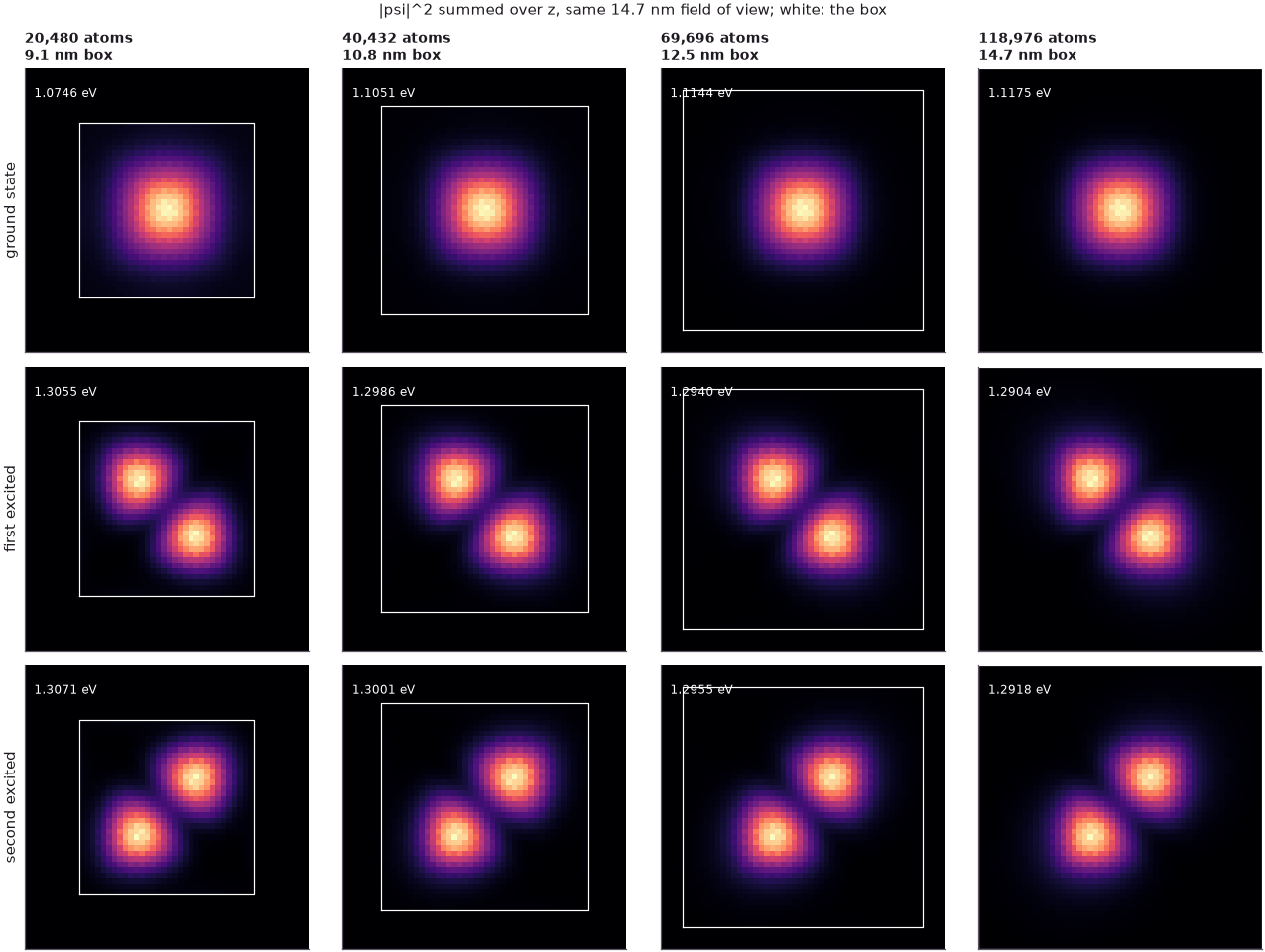
Figure computed by the notebook with open-nemo

The three lowest electron states are found in all four domains, with the same shape: an s-like ground state centred in the pyramid and two p-like states, 1.5 meV apart, with their lobes along the two diagonals of the base, the [110] and [1-10] directions that the zincblende lattice distinguishes. Their energies change from box to box, though, and in opposite directions:

Code15 lines · cell 8

L = np.array([r["n"][0] * a for r in results])
fig, ax = plt.subplots(figsize=(6, 4))
for i, (c, name) in enumerate(zip(style.sweep(nst), ("ground state", "first excited", "second excited"))):
    E = np.array([r["E"][i] for r in results])
    ax.plot(L, E * 1e3 - E[-1] * 1e3, "o-", color=c, label=name)
    print(f"{name:14s}: " + ", ".join(f"{e:.4f}" for e in E) + " eV; change between the two largest boxes "
          f"{(E[-1] - E[-2]) * 1e3:.1f} meV")
ax.axhline(0, color=style.CONTEXT, lw=0.8)
ax.set(xlabel="lateral box size (nm)", ylabel="E − E(largest box) (meV)",
       title="convergence with the buffer size")
ax.legend(frameon=False)
fig.tight_layout()
for r in results:
    print(f"{r['atoms']:6d} atoms: barrier between dot and image {r['n'][0] * a - BASE:5.2f} nm laterally, "
          f"{r['n'][1] * a - HEIGHT:5.2f} nm vertically")

ground state  : 1.0746, 1.1051, 1.1144, 1.1175 eV; change between the two largest boxes 3.1 meV
first excited : 1.3055, 1.2986, 1.2940, 1.2904 eV; change between the two largest boxes -3.6 meV
second excited: 1.3071, 1.3001, 1.2955, 1.2918 eV; change between the two largest boxes -3.7 meV
 20480 atoms: barrier between dot and image  1.07 nm laterally,  2.17 nm vertically
 40432 atoms: barrier between dot and image  2.77 nm laterally,  4.43 nm vertically
 69696 atoms: barrier between dot and image  4.47 nm laterally,  6.70 nm vertically
118976 atoms: barrier between dot and image  6.73 nm laterally,  8.97 nm vertically

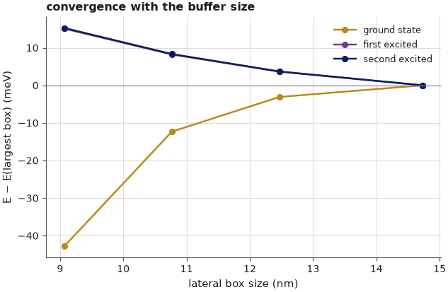
In the smallest box the ground state lies 42.9 meV below its value in the largest one, and the p states 15 meV above. The box is periodic, so the dot is one of a lattice of dots separated by only 1.07 nm of GaAs laterally and 2.17 nm vertically. At \(\mathbf{k} = 0\) the s states of neighbouring dots combine in phase, a bonding combination lowered by the tunnelling between them; the p states, odd along their lobes, combine with the opposite sign across the barrier and are raised. As the buffer grows the coupling decays exponentially, and between the two largest boxes, 4.47 and 6.73 nm of GaAs between dots laterally, the levels move by 3.1 meV (s) and 3.6 meV (p). The test therefore checks two things: the solver extracts the same interior states however large \(H\) is (here up to 594,880 rows), and the buffer must be thick enough for the states to be those of an isolated dot. NEMO 3-D's domains of millions of atoms are large for the second reason too; in a real dot the strain field, which decays more slowly than the wavefunction, sets the size of the mechanical domain (lecture 21.1).

3. What NEMO 3-D can do#

Slide 4: NEMO 3-D capabilities — Slide 4: from atomic orbitals and millions of atoms to the states of artificial atoms and observable quantities; end-to-end wall time grows linearly with the number of atoms, up to 52 million atoms on 128 cores in about 33 hours.

The time per box above also grows with the number of atoms, a little faster than linearly because the number of Lanczos steps rises with the density of states:

Code3 lines · cell 10

for r in results:
    print(f"{r['atoms']:6d} atoms: {r['steps']:4d} Lanczos steps, {r['time']:5.1f} s, "
          f"{r['time'] / r['atoms'] * 1e6:5.1f} us per atom")

 20480 atoms: 1400 Lanczos steps,   4.3 s, 210.0 us per atom
 40432 atoms: 1400 Lanczos steps,   8.4 s, 207.4 us per atom
 69696 atoms: 1600 Lanczos steps,  15.9 s, 227.6 us per atom
118976 atoms: 2000 Lanczos steps,  31.8 s, 266.9 us per atom

The open-nemo counterparts of the capabilities on slide 4 are spread through this book: arbitrary zincblende and wurtzite structures (chapter 2), valence force field strain (lecture 21.2), piezoelectric potentials, empirical tight binding in several bases, and the applications listed on the slide, from InAs/GaAs dots to valley splitting and donors in silicon.

Summary#

Dot states are interior eigenvalues: a few states below the GaAs conduction-band edge inside a spectrum about 26 eV wide (sp3s*) with 100,000 levels or more.
The same InAs pyramid in four periodic GaAs boxes, from 20,480 to 118,976 atoms, gives the same s-like ground state and pair of p-like states, extracted by the Lanczos solver in each case.
The energies converge as the buffer grows, the s level from below (42.9 meV low in the smallest box) and the p levels from above, because the dot couples to its periodic images through thin buffers; between the two largest boxes they still move by 3–4 meV.
NEMO 3-D carried the same test to 21 million atoms and end-to-end calculations to 52 million.

Exercises#

Remove the periodic boundary conditions in \(x\) and \(y\) (passivate the surfaces instead) and repeat the convergence test. Does the ground state approach its limit from above or from below now?
Compute the Bloch phase dependence: evaluate \(H\) at \(\mathbf{k} = (\pi/L, 0, 0)\) for the smallest box. The width of the resulting miniband estimates the tunnel coupling between dots.
Add the Keating relaxation and the strained Hamiltonian of lecture 21.1 for the 19 × 19 × 14 box. How much do strain and the shorter In–As bonds move the levels compared with this unstrained test?