

ECE 606 Lecture 6.3
Electron tunneling — tunneling through a double barrier
In the lecture
- the double barrier as four interfaces: the same transfer-matrix (or scattering-matrix) approach as for one barrier
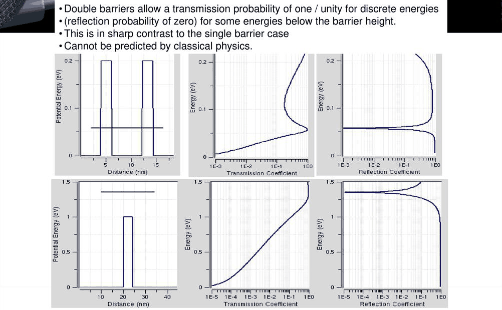
- resonant tunneling: transmission of exactly one at discrete energies below the barrier top
- quasi-bound states above the barrier, with much broader transmission peaks
- taller or thicker barriers sharpen the resonance: the peak width is set by the lifetime of the electron in the well
- comparison with a particle in a box: good for thick, tall barriers, poor for an open system, because the wave function penetrates into the barriers
In this notebook
computes the lecture's PCPBT double-barrier examples with open-nemo, measures the resonance energies and widths (with nemo.resonances and from \(T(E)\)), converts them into lifetimes, compares the widths with a semiclassical escape-rate estimate and the energies with the particle in a box and the finite well, and explores an asymmetric double barrier.
Run it on your own machine
The notebook needs open-nemo (Python ≥ 3.10 and a C++20 compiler; BLAS/LAPACK).
git clone https://github.com/denphi/open-nemo.git && cd open-nemo
python3 -m venv .venv && source .venv/bin/activate
pip install -e ".[notebooks]"
jupyter lab From_Atoms_to_Devices/03_tunneling_and_bandstructure/06_3_double_barrier.ipynbCode
import numpy as np
import matplotlib.pyplot as plt
import opennemo as nemo
from opennemo.visualization import style

style.use(notebook=True)
H2M0 = nemo.core.units.HBAR2_2M0          # ħ²/2m₀ = 0.0381 eV nm²
EM = nemo.structures.materials.EffectiveMassMaterial
1. Four interfaces, one product of matrices#
A double barrier has four interfaces. The transfer-matrix method of Lecture 6.1 handles it without any change: one 2×2 matrix per interface, multiplied in order, and \(T = 1/|M_{11}|^2\) when the contacts on both sides are the same material. The lecture draws the same structure as a cascade of four scattering matrices; either way no particles are lost (\(R + T = 1\)), the incident wave from the left is normalized to one, and nothing is incident from the right. The closed form is a homework problem. Here the product is written out numerically and compared with open-nemo, which solves the discretized Schrödinger equation with open boundaries.
The first example is the lecture's shallow double barrier: two 2 nm barriers of 0.2 eV around a 5 nm GaAs well (effective mass \(m = 0.067\,m_0\) everywhere, \(m_0\) the free-electron mass). The contacts are 10 nm of GaAs on each side.
Code
from scipy.signal import find_peaks, peak_widths

M, DX, LEAD = 0.067, 0.02, 10.0


def double_barrier(b, w, v, b2=None, lead=LEAD, dx=DX):
    """GaAs contacts | barrier b (nm, height v eV) | well w (nm) | barrier b2 (default b) | contacts."""
    gaas, bar = EM("GaAs", M, 12.9), EM("barrier", M, 12.9, conduction_band_edge=v)
    widths = (lead, b, w, b if b2 is None else b2, lead)
    mats = (gaas, bar, gaas, bar, gaas)
    return nemo.Heterostructure1D([nemo.Layer(m, d) for m, d in zip(mats, widths)], spacing=dx)


def tmm_T(E, widths, heights, m=M):
    """T = 1/|M11|² for piecewise-constant layers between two identical contacts at 0 eV."""
    E = np.asarray(E, dtype=complex)
    k = [np.sqrt(m * (E - v) / H2M0 + 0j) for v in (0.0, *heights, 0.0)]
    d = (0.0, *widths)
    total = np.broadcast_to(np.eye(2, dtype=complex), E.shape + (2, 2)).copy()
    for j in range(len(k) - 1):
        kj, kn = k[j], k[j + 1]
        ep, em = np.exp(1j * kj * d[j]), np.exp(-1j * kj * d[j])
        W = np.moveaxis(np.array([[ep, em], [1j * kj * ep, -1j * kj * em]]), (0, 1), (-2, -1))
        Wn = np.moveaxis(
            np.array([[np.ones_like(kn), np.ones_like(kn)], [1j * kn, -1j * kn]]), (0, 1), (-2, -1)
        )
        total = total @ np.linalg.solve(W, Wn)  # interface j: [A_j, B_j] = step · [A_j+1, B_j+1]
    return 1 / np.abs(total[..., 0, 0]) ** 2


E = np.linspace(0.001, 0.6, 6000)
dev = double_barrier(2.0, 5.0, 0.2)
T = nemo.Transport(dev.hamiltonian).transmission(E)
T_tmm = tmm_T(E, (2.0, 5.0, 2.0), (0.2, 0.0, 0.2))
print(f"largest |ln(T open-nemo / T transfer matrix)| = {np.abs(np.log(T / T_tmm)).max():.1e}")
pk = find_peaks(T, prominence=0.05)[0]
for e, t in zip(E[pk], T[pk]):
    print(f"transmission peak at {e:.4f} eV: T = {t:.5f}, R = 1 − T = {1 - t:.1e}")

fig, axes = plt.subplots(1, 3, figsize=(13, 4.2), gridspec_kw={"width_ratios": [0.9, 1, 1]})
axes[0].plot(dev.x - dev.x.mean(), dev.band_edge, color=style.OPEN_NEMO)
for e in E[pk]:
    axes[0].axhline(e, color=style.CONTEXT, ls="--", lw=0.8)
axes[1].semilogx(T, E, color=style.OPEN_NEMO, lw=1.2, label="open-nemo")
axes[1].semilogx(T_tmm, E, ":", color=style.REFERENCE, lw=1, label="transfer matrix")
axes[2].semilogx(1 - T, E, color=style.OPEN_NEMO, lw=1.2)
axes[0].set(
    xlabel="distance from the centre (nm)",
    ylabel="potential energy (eV)",
    ylim=(0, 0.6),
    title="2 nm | 5 nm | 2 nm, 0.2 eV",
)
axes[1].set(xlabel="transmission T", ylabel="energy (eV)", xlim=(1e-3, 2), ylim=(0, 0.6), title="T(E)")
axes[1].legend(frameon=False, fontsize=8)
axes[2].set(xlabel="reflection R = 1 − T", xlim=(1e-6, 2), ylim=(0, 0.6), title="R(E)")
fig.tight_layout();
largest |ln(T open-nemo / T transfer matrix)| = 9.2e-05
transmission peak at 0.0722 eV: T = 1.00000, R = 1 − T = 1.9e-09
transmission peak at 0.3186 eV: T = 1.00000, R = 1 − T = 1.1e-07
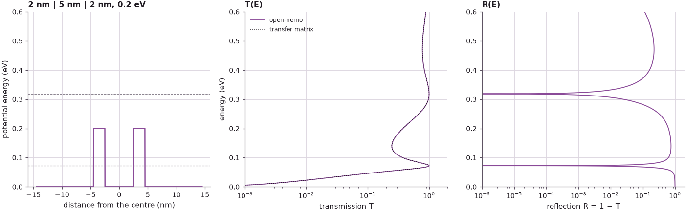
Both methods give the same curve; the small difference is open-nemo's discretization error on the 0.02 nm grid. Two features have no counterpart in the single barrier of Lecture 6.2:
- Resonant tunneling. At 0.072 eV, well below the 0.2 eV barrier top, the transmission is one and the reflection drops to \(2\cdot10^{-9}\) on this energy grid (a deep dip on the logarithmic scale). A single 2 nm barrier of the same height never reaches one below its top. Classically the electron could not cross even one barrier.
- A quasi-bound state above the barriers. At 0.319 eV a second, much broader peak reaches one. The state is only weakly bound: the well "holds" it only by reflection at the barrier edges.
2. Taller and thicker barriers sharpen the resonance#
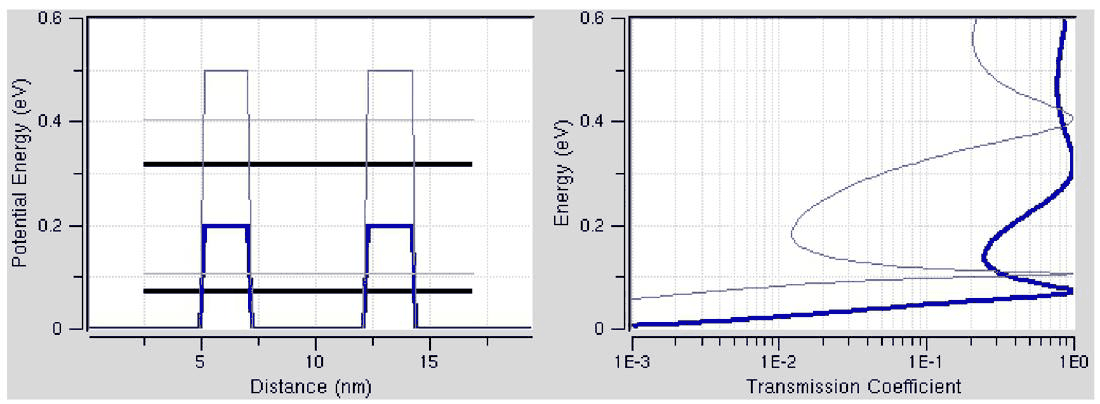
The lecture varies the barriers in two ways: the height, from 0.2 to 0.5 eV at fixed width 2 nm
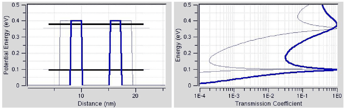
(slide 7), and the thickness, from 2 nm to about 3.5 nm at a height of 0.4 eV (slide 8, read off
the PCPBT figure). For each structure nemo.resonances finds the quasi-bound states as complex
eigenvalues \(E_0 - i\Gamma/2\) of the open-system Hamiltonian; \(E_0\) is the resonance energy and
\(\Gamma\) the full width at half maximum (FWHM) of the transmission peak. The same quantities are
also read directly from the computed \(T(E)\).
Code
HBAR = nemo.core.units.HBAR  # ħ in eV s
cases = [(2.0, 5.0, 0.2), (2.0, 5.0, 0.5), (2.0, 5.0, 0.4), (3.5, 5.0, 0.4)]
E = np.linspace(0.001, 0.6, 6000)
fig, axes = plt.subplots(1, 2, figsize=(11, 4.2), sharey=True)
print(" barrier   height    T peak      FWHM from T   nemo.resonances      lifetime ħ/Γ")
print("  (nm)      (eV)     (eV)          (meV)       E0 (eV)  Γ (meV)        (fs)")
for (b, w, v), ax, lw in zip(cases, (axes[0], axes[0], axes[1], axes[1]), (2.2, 1.0, 2.2, 1.0)):
    dev = double_barrier(b, w, v)
    T = nemo.Transport(dev.hamiltonian).transmission(E)
    res = nemo.resonances(dev)
    pk = find_peaks(T, prominence=0.05)[0]
    for e in E[pk][E[pk] < v]:  # resonances below the barrier top, on a fine grid
        Ef = np.linspace(max(e - 0.08, 0.001), e + 0.08, 8001)
        Tf = nemo.Transport(dev.hamiltonian).transmission(Ef)
        j = np.argmax(Tf)
        fwhm = peak_widths(Tf, [j], rel_height=0.5)[0][0] * (Ef[1] - Ef[0])
        i = np.argmin(np.abs(res["energy"] - Ef[j]))
        print(
            f"  {b:4.1f}     {v:4.2f}     {Ef[j]:.4f}       {fwhm * 1e3:7.3f}      "
            f"{res['energy'][i]:.4f}  {res['width'][i] * 1e3:7.3f}       {HBAR / res['width'][i] * 1e15:6.0f}"
        )
    ax.semilogx(
        T, E, color=style.OPEN_NEMO if lw > 2 else style.sweep(4)[3], lw=lw, label=f"{b:.1f} nm, {v} eV"
    )
    for e in E[pk][E[pk] > v]:
        print(f"  {b:4.1f}     {v:4.2f}     {e:.4f}   above the barrier top (broad quasi-bound state)")
for lead in (10.0, 20.0, 40.0):
    r = nemo.resonances(double_barrier(2.0, 5.0, 0.4, lead=lead))
    print(
        f"2 nm, 0.4 eV, contacts {lead:4.0f} nm: E0 = {np.round(r['energy'], 4)} eV, "
        f"Γ = {np.round(r['width'] * 1e3, 1)} meV"
    )
for ax, title in zip(axes, ("barrier height (2 nm barriers)", "barrier thickness (0.4 eV barriers)")):
    ax.set(xlabel="transmission T", xlim=(1e-4, 2), title=title)
    ax.legend(frameon=False, fontsize=8)
axes[0].set_ylabel("energy (eV)")
fig.tight_layout();
 barrier   height    T peak      FWHM from T   nemo.resonances      lifetime ħ/Γ
  (nm)      (eV)     (eV)          (meV)       E0 (eV)  Γ (meV)        (fs)
   2.0     0.20     0.0722        22.592      0.0691   22.318           29
   2.0     0.20     0.3186   above the barrier top (broad quasi-bound state)
   2.0     0.50     0.1055         6.387      0.1053    6.443          102
   2.0     0.50     0.4054        52.788      0.4038   67.523           10
   2.0     0.40     0.0970         9.723      0.0965    9.828           67
   2.0     0.40     0.3786        63.165      0.3112  153.238            4
   3.5     0.40     0.0995         1.135      0.0995    1.135          580
   3.5     0.40     0.3564        23.202      0.3553   25.436           26
2 nm, 0.4 eV, contacts   10 nm: E0 = [0.0965 0.3112] eV, Γ = [  9.8 153.2] meV
2 nm, 0.4 eV, contacts   20 nm: E0 = [0.0967 0.3618] eV, Γ = [10.3 73.9] meV
2 nm, 0.4 eV, contacts   40 nm: E0 = [0.0965] eV, Γ = [9.6] meV
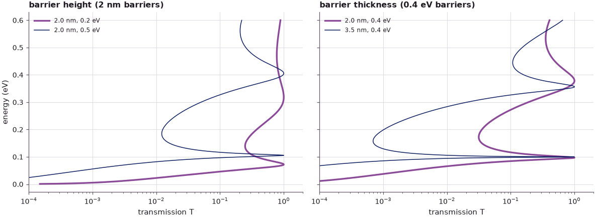
For the lowest resonance the peaks of \(T(E)\) and the complex eigenvalues agree: the widths to within 1.5 %, the energies to within about 3 meV (the transmission maximum sits above \(E_0\) when \(\Gamma\) is large, because the escape rate grows with energy). Raising the barriers from 0.2 to 0.5 eV narrows the lowest resonance from 22 meV to 6.4 meV and pulls a second resonance, at 0.405 eV, below the barrier top: the two strong resonances of slide 7. Thickening the 0.4 eV barriers from 2 to 3.5 nm narrows the lowest resonance by almost a factor of ten, from 9.8 meV to 1.1 meV. The resonance energy moves much less than the width.
The second resonances are broad (23 to 63 meV in \(T\)) and lie close to the barrier top. For them
the transmission peak is the robust quantity. The complex eigenvalue that nemo.resonances
returns for the 2 nm, 0.4 eV structure depends on the length of the contact layers included in the
device: 0.311 eV with 10 nm contacts, 0.362 eV with 20 nm, and no state at all with 40 nm, while
the transmission peak stays at 0.379 eV. Even the narrow lowest state changes its width by about 7 % (9.6 to 10.3 meV)
between these contact lengths.
3. Resonance width and lifetime#
Klimeck describes the double barrier as a resonator: an electron placed in the well bounces between the barriers and eventually leaks out. If \(\tau\) is its lifetime, the energy of the state is uncertain by \(\Gamma = \hbar/\tau\), and the transmission near the resonance is a Lorentzian,
where \(\Gamma_L\) and \(\Gamma_R\) are the escape rates (times \(\hbar\)) through the left and right barrier. The table above converts the widths: 30 fs for the shallow structure, 580 fs for the thick barriers.
A semiclassical estimate makes the dependence on the barriers explicit. The electron moves in the well with velocity \(v = \hbar k/m\); it hits one barrier every \(2W_\mathrm{eff}/v\) seconds and escapes with the single-barrier probability \(T_1(E)\) of Lecture 6.2 each time:
\(W\) is the well width and \(W_\mathrm{eff}\) adds the decay length \(1/\gamma\) of the wave function
into each barrier (Section 5). The estimate uses the resonance energy \(E_0\) from nemo.resonances.
Code
def t_single(E, L, V0, m=M):
    """Exact single-barrier transmission (Lecture 6.2)."""
    k, g = np.sqrt(m * E / H2M0 + 0j), np.sqrt(m * (V0 - E) / H2M0 + 0j)
    return (1 / (1 + ((g**2 + k**2) / (2 * k * g)) ** 2 * np.sinh(g * L) ** 2)).real


print(" barrier  height   E0 (eV)   Γ open-nemo (meV)   Γ estimate (meV)   T1 single barrier")
for b, w, v in cases:
    res = nemo.resonances(double_barrier(b, w, v))
    E0, G = res["energy"][0], res["width"][0]
    k, g = np.sqrt(M * E0 / H2M0), np.sqrt(M * (v - E0) / H2M0)
    hbar_v = 2 * H2M0 * k / M  # ħv = ħ²k/m in eV nm
    T1 = t_single(E0, b, v)
    G_est = hbar_v / (2 * (w + 2 / g)) * 2 * T1
    print(
        f"  {b:4.1f}    {v:4.2f}    {E0:.4f}        {G * 1e3:7.3f}            {G_est * 1e3:7.3f}         "
        f" {T1:.3e}"
    )
 barrier  height   E0 (eV)   Γ open-nemo (meV)   Γ estimate (meV)   T1 single barrier
   2.0    0.20    0.0691         22.318             18.239          4.218e-01
   2.0    0.50    0.1053          6.443              6.129          9.268e-02
   2.0    0.40    0.0965          9.828              9.067          1.497e-01
   3.5    0.40    0.0995          1.135              1.125          1.833e-02
The escape-rate estimate is within about 20 % for the shallow 0.2 eV structure and within 8 % for the others (1 % for the thick barriers), with no adjustable parameter. It explains the trends of slides 7 and 8: the width is proportional to the single-barrier transmission, which falls exponentially with the barrier thickness and with \(\sqrt{V_0 - E}\) (Lecture 6.2). A sharper resonance means a longer residence time in the well.
4. The well as a particle in a box#
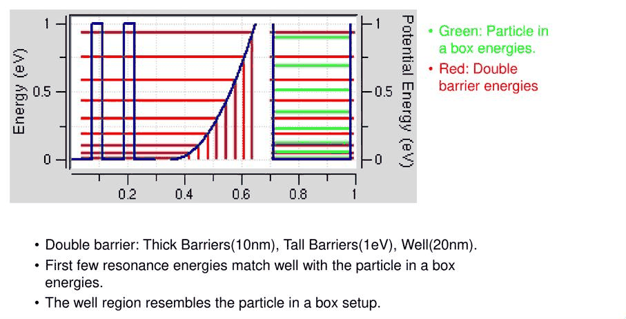
If the barriers confine the electron well, the resonances should be close to the levels of a particle in a box (Lecture slide 10) of width \(W\),
A better closed model is the finite square well of depth \(V_0\): the same well, but with barriers that extend to infinity, so that the wave function decays into them without leaking out. Its levels solve \(\tan(kW/2) = \gamma/k\) (even states) and \(-\cot(kW/2) = \gamma/k\) (odd states). The lecture compares two structures: thick, tall barriers (10 nm, 1 eV, 20 nm well; slide 11) and thinner, lower ones (8 nm, 0.25 eV, 10 nm well; slide 12).
Code
from scipy.optimize import brentq


def finite_well_levels(W, V0, m=M):
    """Bound states of a square well of width W (nm) and depth V0 (eV), barriers infinitely thick."""
    f_even = lambda e: np.sqrt(e) * np.tan(np.sqrt(m * e / H2M0) * W / 2) - np.sqrt(V0 - e)
    f_odd = lambda e: -np.sqrt(e) / np.tan(np.sqrt(m * e / H2M0) * W / 2) - np.sqrt(V0 - e)
    grid = np.linspace(1e-6, V0 - 1e-9, 20001)
    levels = []
    for f in (f_even, f_odd):
        y = f(grid)
        for i in np.nonzero((np.sign(y[:-1]) != np.sign(y[1:])) & (np.abs(y[:-1] - y[1:]) < 1))[0]:
            levels.append(brentq(f, grid[i], grid[i + 1]))
    return np.sort(levels)


fig, axes = plt.subplots(1, 2, figsize=(11, 4.4))
for (b, w, v), ax in zip(((10.0, 20.0, 1.0), (8.0, 10.0, 0.25)), axes):
    res = nemo.resonances(double_barrier(b, w, v))
    E0 = res["energy"][res["energy"] < v]
    well = finite_well_levels(w, v)
    n = np.arange(1, len(E0) + 1)
    box = H2M0 * np.pi**2 * n**2 / (M * w**2)
    print(f"{b:.0f} nm, {v} eV barriers, {w:.0f} nm well")
    print("   n   resonance (eV)   width Γ (eV)   finite well (eV)   particle in a box (eV)   ratio E0/E_box")
    for j in range(len(E0)):
        print(
            f"  {n[j]:2d}     {E0[j]:.5f}       {res['width'][j]:.1e}         {well[j]:.5f}"
            f"              {box[j]:.5f}               {E0[j] / box[j]:.3f}"
        )
    ax.plot(n, box, "s", mfc="none", color=style.CONTEXT, label="particle in a box (closed)")
    ax.plot(n, well[: len(n)], "x", color=style.REFERENCE, label="finite well (closed)")
    ax.plot(n, E0, "o", ms=4, color=style.OPEN_NEMO, label="double-barrier resonance (open-nemo)")
    ax.axhline(v, color=style.CONTEXT, ls=":", lw=0.8)
    ax.set(
        xlabel="level n",
        ylabel="energy (eV)",
        xticks=n,
        title=f"{b:.0f} nm, {v} eV barriers, {w:.0f} nm well",
    )
    ax.legend(frameon=False, fontsize=8)
fig.tight_layout();
10 nm, 1.0 eV barriers, 20 nm well
   n   resonance (eV)   width Γ (eV)   finite well (eV)   particle in a box (eV)   ratio E0/E_box
   1     0.01213       5.3e-15         0.01213              0.01403               0.864
   2     0.04847       6.6e-14         0.04847              0.05612               0.864
   3     0.10890       4.8e-13         0.10890              0.12628               0.862
   4     0.19315       3.4e-12         0.19316              0.22450               0.860
   5     0.30083       3.0e-11         0.30083              0.35077               0.858
   6     0.43123       3.6e-10         0.43124              0.50512               0.854
   7     0.58313       7.3e-09         0.58315              0.68752               0.848
   8     0.75392       3.3e-07         0.75395              0.89798               0.840
   9     0.93517       6.4e-05         0.93516              1.13651               0.823
8 nm, 0.25 eV barriers, 10 nm well
   n   resonance (eV)   width Γ (eV)   finite well (eV)   particle in a box (eV)   ratio E0/E_box
   1     0.03277       1.9e-06         0.03277              0.05612               0.584
   2     0.12589       8.5e-05         0.12590              0.22450               0.561
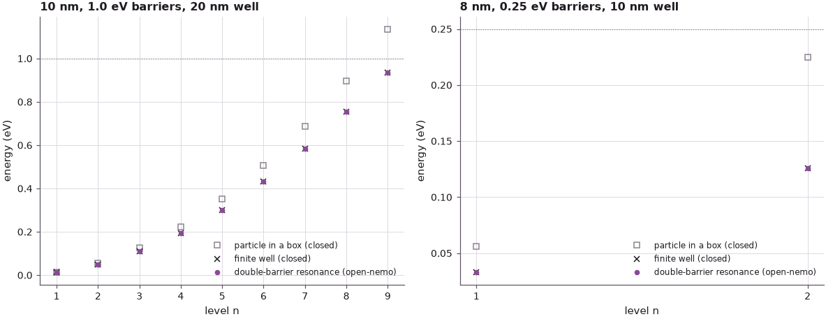
For the thick, tall barriers the lowest resonances lie 14 % below the particle-in-a-box levels, the discrepancy grows towards the barrier top, and the widths are tiny: \(5\cdot10^{-15}\) eV for the ground state, a lifetime of the order of a tenth of a second. For the thinner, lower barriers even the ground state lies at 0.6 of the box energy, as the lecture states: "the system doesn't resemble very well anymore the particle in a box problem".
The finite well, by contrast, reproduces every resonance to within 0.03 meV in both structures. What the infinite box misses is not the openness itself (the widths are far smaller than the level spacings) but the finite barrier height: the wave function leaks into the barriers, which makes the box effectively wider and lowers the levels. Openness matters for the width, and for the energy only when the width becomes comparable to the spacing.
5. Penetration into the barriers and the effective well width#
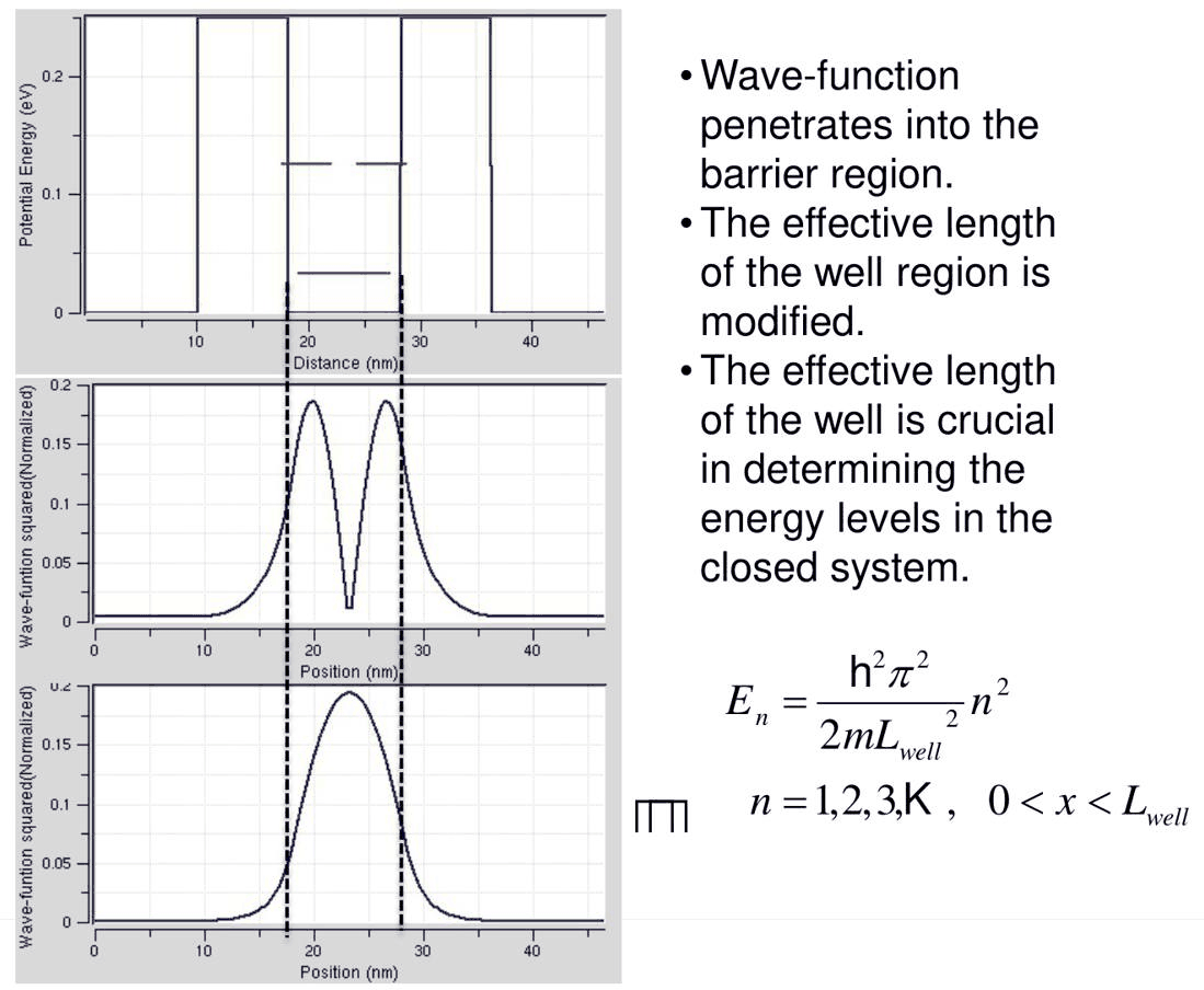
The lecture's slide 13 plots \(|\psi|^2\) of the two resonances of the 8 nm, 0.25 eV structure,
computed with tight binding in the tool. nemo.resonances returns the same densities, normalized
over the device. The fraction of the density inside the barriers measures the penetration, and an
effective width \(W_\mathrm{eff} = \pi n\,\hbar/\sqrt{2mE_0}\) makes the box formula reproduce each
resonance exactly.
Code
b, w, v = 8.0, 10.0, 0.25
dev = double_barrier(b, w, v)
res = nemo.resonances(dev)
x = dev.x - dev.x.mean()
in_barrier = (np.abs(x) > w / 2) & (np.abs(x) < w / 2 + b)
fig, (a1, a2) = plt.subplots(2, 1, figsize=(7.5, 6), sharex=True, gridspec_kw={"height_ratios": [1, 1.4]})
a1.plot(x, dev.band_edge, color=style.CONTEXT)
for n, (E0, rho, c) in enumerate(zip(res["energy"][:2], res["density"][:2], style.sweep(2)), start=1):
    k, g = np.sqrt(M * E0 / H2M0), np.sqrt(M * (v - E0) / H2M0)
    w_eff = np.pi * n / k
    print(
        f"n = {n}: E0 = {E0:.4f} eV, density in the barriers = {rho[in_barrier].sum():.3f}, "
        f"W_eff = {w_eff:.2f} nm, W + 2/γ = {w + 2 / g:.2f} nm"
    )
    a1.hlines(E0, -w / 2, w / 2, color=c, lw=1.6)
    a2.plot(x, rho / DX, color=c, label=f"n = {n}, E = {E0:.3f} eV")
for ax in (a1, a2):
    for s in (-w / 2, w / 2):
        ax.axvline(s, color=style.CONTEXT, ls="--", lw=0.7)
a1.set(ylabel="potential energy (eV)", title="8 nm, 0.25 eV barriers around a 10 nm well")
a2.set(xlabel="distance from the centre (nm)", ylabel="|ψ|² (1/nm)", xlim=(-20, 20))
a2.legend(frameon=False, fontsize=8)
fig.tight_layout();
n = 1: E0 = 0.0328 eV, density in the barriers = 0.032, W_eff = 13.09 nm, W + 2/γ = 13.24 nm
n = 2: E0 = 0.1259 eV, density in the barriers = 0.151, W_eff = 13.35 nm, W + 2/γ = 14.28 nm
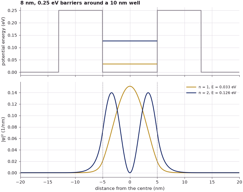
The ground state places 3 % of its density inside the barriers and the first excited state, which sits closer to the barrier top, 15 %. Measured by its energy, the ground state behaves like a particle in a box 13.1 nm wide instead of 10 nm; the excited state behaves like one 13.4 nm wide. The simple estimate \(W + 2/\gamma\), one decay length added on each side, gives 13.2 nm and 14.3 nm: good for the deep state, too large for the shallow one. Klimeck's remark that one can "play some number games to make them match" applies: an effective width can be fitted level by level, but it is a different width for each level, which is why the finite-well or the open-system calculation is the reliable route.
6. Exploration: an asymmetric double barrier#
In the symmetric structure the peak transmission is exactly one. If the two barriers differ, the Lorentzian of Section 3 gives at \(E = E_0\)
using the escape-rate estimate \(\Gamma_{L,R} \propto T_1^{L,R}\). The left barrier is kept at 2 nm and the right one is thickened, at 0.4 eV around a 5 nm well.
Code
print(" right barrier (nm)   E0 (eV)   Γ (meV)   T peak open-nemo   4 T1L T1R / (T1L + T1R)²")
fig, ax = plt.subplots(figsize=(7.5, 4))
for b2, c in zip((2.0, 2.5, 3.0, 4.0), style.sweep(4)):
    dev = double_barrier(2.0, 5.0, 0.4, b2=b2)
    res = nemo.resonances(dev)
    E0 = res["energy"][0]
    Ef = np.linspace(E0 - 0.03, E0 + 0.03, 6001)
    T = nemo.Transport(dev.hamiltonian).transmission(Ef)
    tl, tr = t_single(E0, 2.0, 0.4), t_single(E0, b2, 0.4)
    print(
        f"        {b2:3.1f}          {E0:.4f}    {res['width'][0] * 1e3:6.3f}      {T.max():.4f}"
        f"              {4 * tl * tr / (tl + tr) ** 2:.4f}"
    )
    ax.plot(Ef, T, color=c, label=f"2 nm | 5 nm | {b2} nm")
ax.set(xlabel="E (eV)", ylabel="T(E)", title="asymmetric double barrier, 0.4 eV")
ax.legend(frameon=False, fontsize=8);
 right barrier (nm)   E0 (eV)   Γ (meV)   T peak open-nemo   4 T1L T1R / (T1L + T1R)²
        2.0          0.0965     9.828      1.0000              1.0000
        2.5          0.0975     7.362      0.8738              0.8863
        3.0          0.0979     6.173      0.6049              0.6284
        4.0          0.0982     5.323      0.1910              0.2044
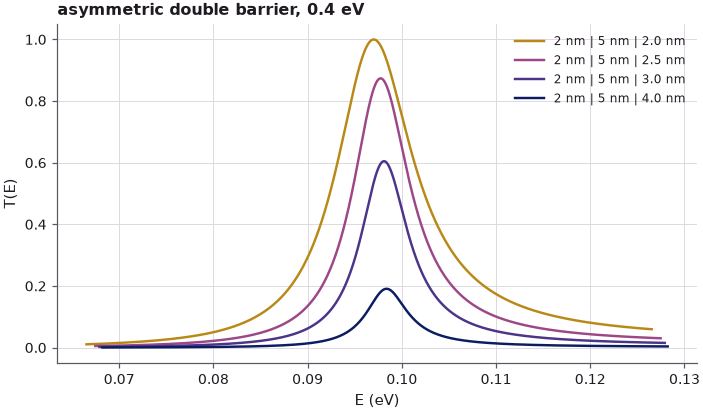
With a thicker right barrier the peak falls below one, to 0.60 at 3 nm and 0.19 at 4 nm, and the estimate from the two single-barrier transmissions follows the computed peaks to within 0.03. The resonance also narrows, from 9.8 to 5.3 meV, but only to about half: the total escape rate becomes dominated by the 2 nm barrier alone, which keeps its share \(\Gamma_L\). Unit transmission requires matched barriers: the reflected waves from the two sides cancel only when the electron leaks out of the well equally fast in both directions.
Summary#
- A double barrier is four interfaces; the transfer matrix (or scattering matrix) handles it in the same way as one barrier, and open-nemo's open-boundary transmission agrees with it.
- It transmits with probability one at discrete energies below the barrier top (resonant tunneling), which neither a single barrier nor classical physics allows. Above the top it has broad, weakly bound states.
- Each resonance is a quasi-bound state \(E_0 - i\Gamma/2\) with a finite lifetime \(\tau = \hbar/\Gamma\). Taller or thicker barriers lengthen the lifetime and sharpen the peak, in proportion to the single-barrier transmission: \(\Gamma \approx (\hbar v/2W_\mathrm{eff})(T_1^L + T_1^R)\).
- The particle in a box overestimates the resonance energies because the wave function penetrates into the barriers; the finite well reproduces them as long as the width is small compared with the level spacing.
- Unequal barriers lower the peak transmission to \(4\Gamma_L\Gamma_R/(\Gamma_L + \Gamma_R)^2\).
Exercises#
- For the 2 nm | 5 nm | 2 nm structure, find the barrier height at which the lowest resonance
width equals 1 meV, first with the escape-rate estimate and then with
nemo.resonances. - Fit the Lorentzian of Section 3 to the computed \(T(E)\) of the 3.5 nm, 0.4 eV structure. How far from \(E_0\) does the Lorentzian stay within 10 % of \(T\)?
- Make the barriers of the 8 nm, 0.25 eV structure out of a material with mass \(0.1\,m_0\). Predict the direction of the change of \(E_0\) and \(\Gamma\) before computing them.
- Repeat Section 6 with equal widths but unequal heights (0.3 and 0.5 eV). Which barrier controls the width of the resonance?
Further reading#
- Lecture 6.2: the single barrier and Lecture 6.4: N barriers and the formation of bands.
- The resonant-tunneling diode tutorial: the resonant-tunneling diode built from the same double barrier.
- Benchmark: piecewise-constant barriers against nanoHUB's PCPBT.
- The tool of the lecture: PCPBT on nanoHUB.