Electron tunneling — the transfer matrix method

1. From a closed box to an open system#

Section 5 solved closed problems: an electron in an infinite or finite well. The recipe had five steps:

1. write a solution ansatz in each of the \(N\) regions of constant potential (\(2N\) unknown coefficients),
2. impose \(\psi(\pm\infty) = 0\) at the two outer edges (2 unknowns fewer),
3. impose continuity of \(\psi\) and \(d\psi/dx\) at every interface (\(2N-2\) equations),
4. set the determinant of the coefficient matrix to zero, which selects the allowed energies,
5. normalize \(\int|\psi|^2dx = 1\) to fix the last coefficient.

A tunneling problem is different: the electron comes in from one contact and may leave through the other. Every energy is allowed, so step 4 disappears, and the wave extends to infinity, so step 5 disappears too. Step 2 is replaced by an open boundary condition: we fix what comes in. The interface conditions of step 3 are unchanged, and they are all the physics there is.

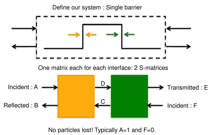
Klimeck draws the single barrier as a two-port network, familiar from circuit analysis: each interface is a box that couples a wave coming in and a wave going out on each side. A wave of amplitude \(A\) is incident from the left, \(B\) is reflected, \(E\) is transmitted; \(C\) and \(D\) live inside the barrier. Usually nothing is injected from the right, \(F = 0\), and the incident wave is normalized, \(A = 1\). That removes two unknowns, and no particles are lost: what is not transmitted is reflected.

2. The three regions of a single barrier#

A barrier of height \(V_0\) and width \(L\) sits between \(x = 0\) and \(x = L\). The energy is measured from the conduction-band edge of the two outer regions. An electron of energy \(E < V_0\) is classically allowed in regions 1 and 3 and forbidden in region 2. The effective-mass Schrödinger equation \(d^2\psi/dx^2 + k^2\psi = 0\) has the solutions

As the lecture stresses, \(k\) and \(\gamma\) are the same object: each is measured from the band edge of its own region, upwards for \(k\), downwards from the barrier top for \(\gamma\). Inside the barrier the wave number is imaginary, \(k_2 = i\gamma\).

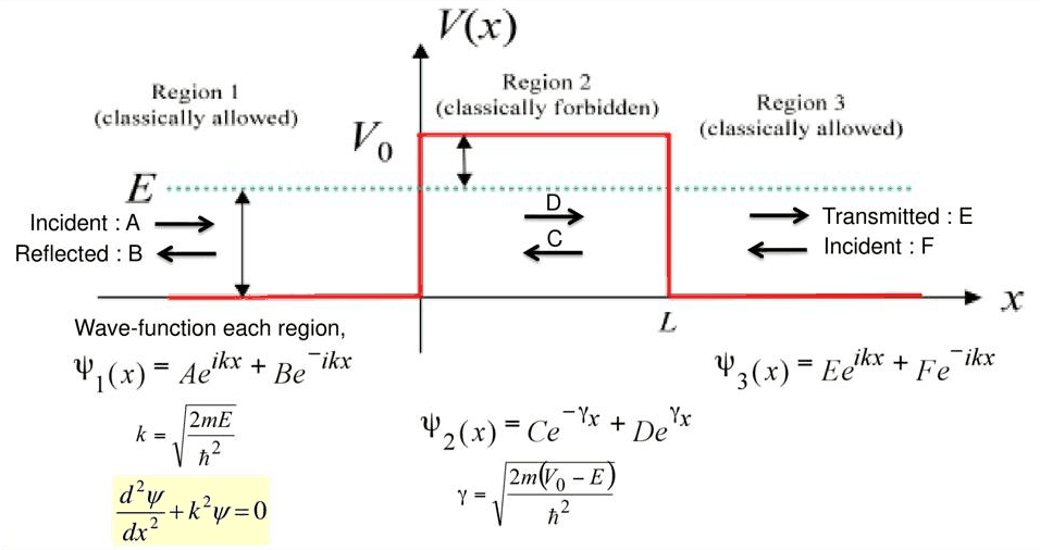
The barrier material has its own band structure, \(E = V_0 + \hbar^2k^2/2m\). At an energy below its edge, its Bloch "waves" have a complex wave number: these are the evanescent states that the ansatz \(e^{\pm\gamma x}\) describes. open-nemo's complex_bands computes them for the discretized barrier material (a chain of sites with spacing \(a\)); its imaginary wave number is the decay constant \(\gamma\). Throughout this notebook the mass is GaAs's, \(m = 0.067\,m_0\), and the barrier is \(V_0 = 0.4\) eV high.

The decay constants agree to the fourth digit; the small difference is the grid (\(a = 0.01\) nm): a discretized chain has \(\cosh(\gamma a) = 1 + (V_0 - E)/2t_0\) rather than \(\gamma^2 = (V_0-E)/t_0a^2\). The decay length \(1/\gamma\) is about a nanometre: a barrier a few nanometres wide is crossed by an amplitude that has dropped by \(e^{-\gamma L}\), small but not zero. That is tunneling.

3. The interface conditions as matrices#

At \(x = 0\) continuity of \(\psi\) and \(\psi'\) gives \(A + B = C + D\) and \(ik(A - B) = -\gamma(C - D)\); at \(x = L\) the same two conditions connect \(C, D\) with \(E, F\). Each pair can be solved for the amplitudes on the left, which gives two 2×2 matrices:

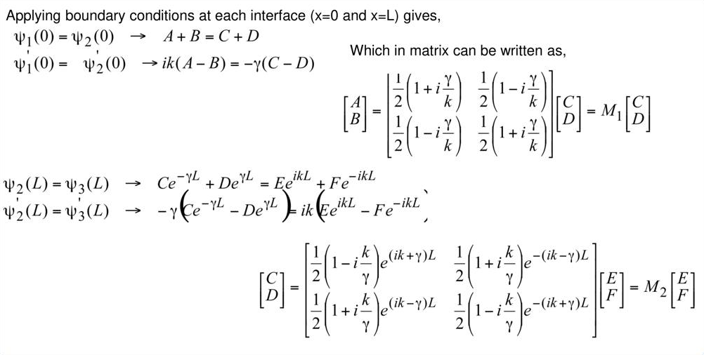
Chaining the two, \([A, B]^T = M_1 M_2 [E, F]^T = M [E, F]^T\). With \(F = 0\) the first row reads \(A = M_{11}E\), so the transmitted amplitude is \(t = E/A = 1/M_{11}\), the reflected one \(r = B/A = M_{21}/M_{11}\), and the transmission is

The cell below codes \(M_1\) and \(M_2\) exactly as printed on the slide. Above the barrier the same formulas hold with \(\gamma = \sqrt{2m(V_0 - E)}/\hbar\) imaginary, so one function covers all energies.

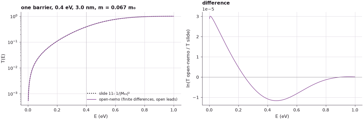
The two transmissions lie on top of each other, from \(5\cdot10^{-4}\) at 2 meV to 0.39 at the barrier top. \(T\) is far from zero below the top and, as the next lecture shows, still below one above it: there is no sharp classical threshold (the subject of the next lecture). The matrices conserve the current: reflection and transmission add up to one to round-off. The remaining difference, at most \(3\cdot10^{-5}\) in \(\ln T\), is the discretization of open-nemo's grid, which grows with energy because the error of the three-point second derivative scales as \((ka)^2\) (Lecture 6.5).

4. The general transfer-matrix method#

Nothing in this construction is special to one barrier. For any stack of layers \(j = 1 \dots N\) of constant potential \(V_j\) and mass \(m_j\), write in each layer

(real or imaginary), with \(x_j\) the left edge of the layer. Continuity of \(\psi\) and of the flux \(\psi'/m\) (the BenDaniel–Duke condition, needed when the mass changes from layer to layer) at each interface gives one 2×2 matrix per interface, and

With \(A_1^+ = 1\) and \(A_N^- = 0\) the transmission is \(T = \frac{k_N/m_N}{k_1/m_1}\,|1/M_{11}|^2\): the prefactor is the ratio of the group velocities in the two contacts, which is 1 when they are the same material. The function below implements this for many energies at once, and the first check is that it reproduces the slide's \(M_1M_2\).

Same matrices, once the phase convention is matched: the slide counts the phase of \(E\) and \(F\) from \(x = 0\), the general code from the right interface \(x = L\), which multiplies \(E\) by \(e^{ikL}\) and leaves \(|M_{11}|\), and \(T\), unchanged. The homework the lecture suggests is the double barrier: four interfaces instead of two. Here it is computed both ways, together with a heterostructure in which the barrier has a heavier mass (\(0.092\,m_0\), as in AlGaAs) and the right contact sits 0.1 eV lower than the left one, so that all three ingredients of the general formula (complex \(k_j\), the mass in the flux, the velocity ratio) are exercised.

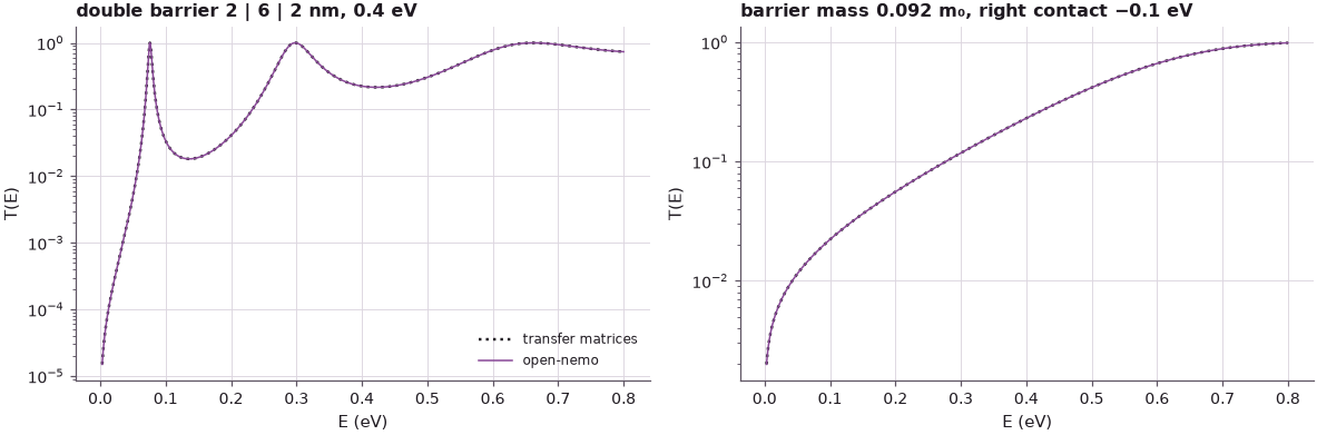
The double barrier transmits completely, \(T = 1\), at an energy well below the barrier top: resonant tunneling, the topic of Lecture 6.3. The largest differences sit on the flanks of that sharp peak, where a tiny shift of the peak energy changes \(T\) a lot; the median difference is \(2\cdot10^{-5}\). In the heterostructure, waves enter only above the left contact's edge (\(E = 0\)), and the step between the two contacts reflects part of the wave even far above the barrier, so \(T\) stays below one there.

The difference between the two methods is open-nemo's grid. Halving the spacing should divide it by four:

It does: the finite-difference solution converges to the transfer-matrix one as \(a^2\). For piecewise constant potentials the transfer matrices are exact, and they are an excellent check on any numerical code.

5. The wave function from the coefficients#

The transfer matrix gives more than \(T\): once \(E = t\) is known, \([A_j^+, A_j^-]\) follows in every layer, and with it \(\psi(x)\). Below, the single barrier at \(E = 0.2\) eV (half the barrier height). open-nemo returns the density injected from the left contact (spectral_left, the diagonal of \(G\Gamma_LG^\dagger\)), which is \(|\psi|^2\) of the same scattering state up to a constant; it is scaled here so that it equals \(|t|^2\) in the right contact.

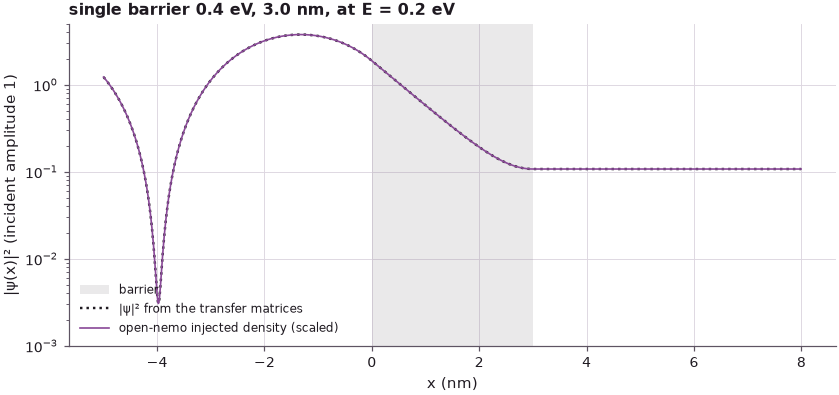
On the left, the incident and reflected waves interfere: \(|\psi|^2 = |e^{ikx} + re^{-ikx}|^2\) oscillates between \((1-|r|)^2\) and \((1+|r|)^2\), almost a standing wave because \(|r|^2\) is close to one. Inside the barrier the density falls exponentially, mostly through \(C e^{-\gamma x}\); the growing term \(De^{\gamma x}\) has a tiny coefficient and only bends the curve near \(x = L\), where it is needed to match the outgoing wave. On the right only the transmitted wave remains, with the constant density \(|t|^2\). The two methods give the same state.

6. Simple and pleasing, with a catch#

The lecture calls the method "conceptually very simple and analytically pleasing", and recommends it for the double-barrier homework, but warns that it has numerical issues. The cause is visible in the matrices: an evanescent layer contributes \(e^{+\gamma d}\) and \(e^{-\gamma d}\) to the same product. The size of \(M_{11}\) grows exponentially with the barrier width, and every quantity that results from a cancellation between such terms keeps only the digits left over by floating-point arithmetic (about 16).

The transfer matrix between two identical contacts has determinant exactly 1 (current conservation), yet its elements grow like \(e^{\gamma L}\). The determinant is the difference of two products of size \(|M_{11}|^2\): as computed, it keeps fewer and fewer correct digits as the barrier widens, and when \(|M_{11}|^2\) approaches \(10^{16}\) none are left (the last rows of the table). For a single barrier \(T = 1/|M_{11}|^2\) is still accurate, because no cancellation is needed. For many layers, for the wave function deep inside thick barriers, or for a resonance that needs a large \(M_{11}\) to cancel down to one, the precision is lost. Lecture 6.5 returns to this, and to the discretized Schrödinger equation that open-nemo solves instead.

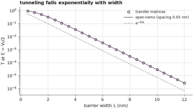
Every nanometre of barrier costs the same factor, \(e^{-2\gamma\cdot 1\,\text{nm}}\), once the barrier is wider than about one decay length: the exponential law that Lecture 6.2 derives from the exact formula. The dotted line has that slope; the curves lie above it by the prefactor \((4k\gamma/(k^2+\gamma^2))^2\), which is 4 at \(E = V_0/2\), where \(k = \gamma\).

Summary#

• An open system differs from a closed one only in its boundary conditions: the incident amplitude is fixed (\(A = 1\), \(F = 0\)), every energy is allowed, and there is no normalization.
• In each region of constant potential the solution is \(e^{\pm ikx}\) (allowed) or \(e^{\pm\gamma x}\) (forbidden, \(k = i\gamma\)); \(\gamma\) is the imaginary wave number of the barrier's complex band structure.
• Continuity of \(\psi\) and \(\psi'/m\) at each interface is a 2×2 matrix; their product is the transfer matrix \(M\), and \(T = (v_N/v_1)/|M_{11}|^2\).
• The slide's \(M_1M_2\), a general transfer-matrix code and open-nemo's finite-difference transport agree; the latter converges as \(a^2\) to the exact piecewise-constant result. The wave function rebuilt from the coefficients is open-nemo's injected density.
• The matrix elements grow as \(e^{\gamma L}\) while \(\det M = 1\): the method loses precision when large terms must cancel.

Exercises#

1. Use tmm_transmission to compute \(T(E)\) of a double barrier with 3 nm barriers and a 5 nm well, and find the energy of the transmission peak. Compare with nemo.resonances(device(...)).
2. Make the right contact 0.2 eV lower than the left one (a step) and remove the barrier. Check that \(R + T = 1\) when \(T\) includes the velocity ratio, and that it fails without it.
3. Plot \(|\psi(x)|^2\) for the single barrier at \(E = 0.6\) eV, above the barrier. What replaces the exponential decay inside it?
4. Repeat the table of section 6 at \(E = 0.39\) eV. Why does \(M_{11}\) grow so much more slowly?

Further reading#

• Quantum transport from scratch: Green's functions on a 1-D chain: the open boundary conditions that open-nemo uses instead of transfer matrices.
• Benchmark: piecewise-constant barriers against nanoHUB's PCPBT: open-nemo against the transfer-matrix tool used throughout Section 6.
• Resonant tunneling diode, step by step.
• The tool of the lecture: Piece-Wise Constant Potential Barriers Tool (PCPBT) on nanoHUB.
• The numerical limits of transfer matrices and better methods: G. Klimeck, Nanoelectronic Modeling: From Quantum Mechanics and Atoms to Realistic Devices, nanoHUB resource 8086 (2010).