Course/03 · Tunneling and band structure

ECE 606 Lecture 7.2

Band structure in a periodic potential — solutions

In the lecture

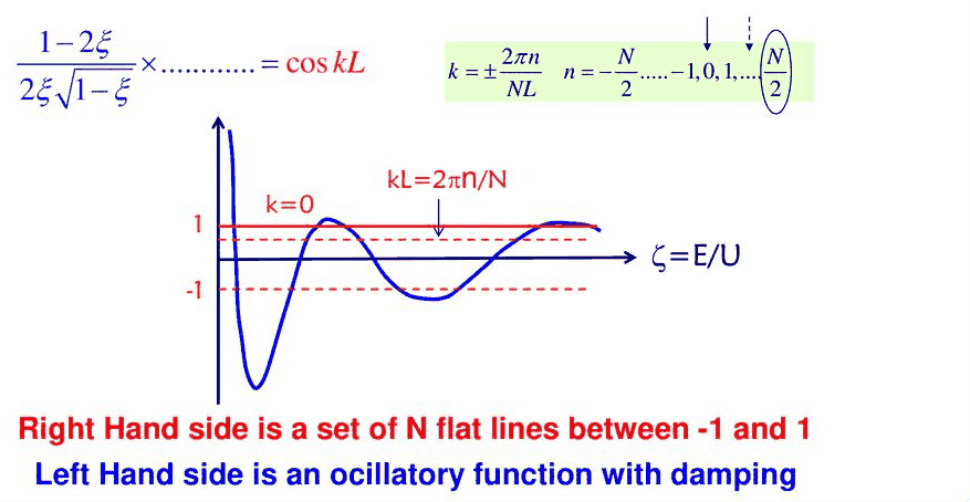
the graphical solution of \(\cos kL = f(\xi)\): \(N\) flat lines between −1 and 1 against an oscillating, damped function of \(\xi = E/U_0\)
allowed bands and forbidden gaps, and the band diagram \(E(k)\)
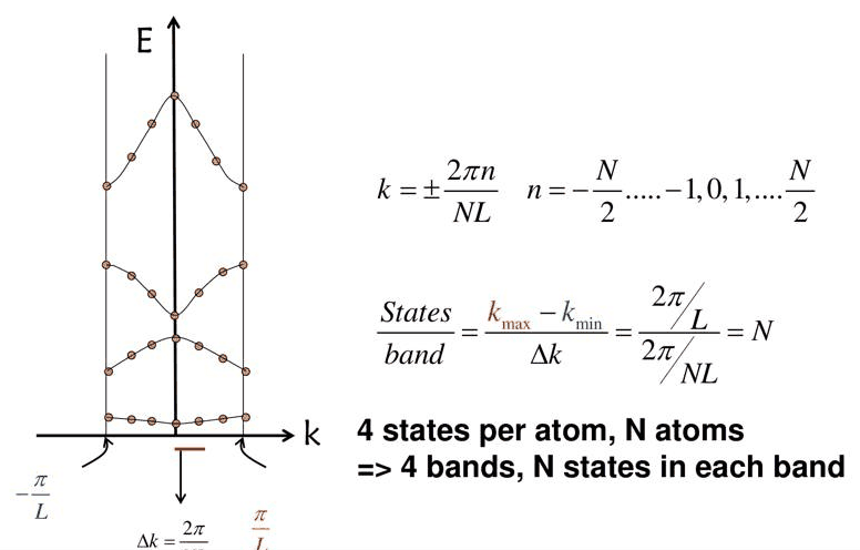
the Brillouin zone \(-\pi/L \le k \le \pi/L\), the spacing \(\Delta k = 2\pi/(NL)\) and \(N\) states per band
comparison with finite superlattices of 30 and 80 barriers (tight binding and transfer matrices in PCPBT) and the periodic model (Periodic Potential Lab), for GaAs and InAs
a finite superlattice with many cells approaches the periodic potential model

In this notebook

solves the Kronig–Penney equation graphically and numerically, draws the bands in the reduced and extended zones, counts the states per band in rings of \(N\) cells, reproduces the lecture's GaAs and InAs comparisons of 30- and 80-barrier structures (open-nemo transmission and an analytic transfer matrix) with the periodic bands, and explores how weak barriers open gaps.

Run the notebookEvery number and figure on this page comes from it. Change it, rerun it, take it further.

Download .ipynb View on GitHub

Run it on your own machine

The notebook needs open-nemo (Python ≥ 3.10 and a C++20 compiler; BLAS/LAPACK).

git clone https://github.com/denphi/open-nemo.git && cd open-nemo
python3 -m venv .venv && source .venv/bin/activate
pip install -e ".[notebooks]"
jupyter lab From_Atoms_to_Devices/03_tunneling_and_bandstructure/07_2_bandstructure_solutions.ipynb

Code8 lines · cell 1

import numpy as np
import matplotlib.pyplot as plt
import opennemo as nemo
from opennemo.visualization import style

style.use(notebook=True)
H2M0 = nemo.core.units.HBAR2_2M0          # ħ²/2m₀ = 0.0381 eV nm²
EM = nemo.structures.materials.EffectiveMassMaterial

1. The graphical solution#

Lecture 7.1 reduced the periodic problem to one equation,

\cos kL = f(\xi), \qquad \xi = \frac{E}{U_0}, \qquad k = \frac{2\pi n}{NL},\quad n = -\frac N2, \dots, \frac N2 - 1,

where \(f\) is the Kronig–Penney function of the cell (a well of width \(a\), a barrier of width \(b\) and height \(U_0\), period \(L = a + b\)) and \(N\) is the number of cells in the ring that closes the periodic structure. The right-hand side takes only \(N\) values, "a set of \(N\) flat lines between −1 and 1"; the left-hand side "is an oscillatory function with damping". Each intersection is a state. The structure is the lecture's GaAs example: \(a = 6\) nm, \(b = 2\) nm, \(U_0 = 0.4\) eV, \(m = 0.067\,m_0\).

Slide 3: graphical solution to the energy levels — Slide 3: the flat lines \(\cos(2\pi n/N)\) (red) and the oscillating function \(f(\xi)\) (blue).

Code43 lines · cell 3

from scipy.optimize import brentq

M, A, B, U0 = 0.067, 6.0, 2.0, 0.4
L = A + B


def kp_f(E, m=M, a=A, b=B, U=U0):
    """Kronig–Penney function: cos kL = f(E), valid below and above the barrier top."""
    al, be = np.sqrt(m * E / H2M0 + 0j), np.sqrt(m * (E - U) / H2M0 + 0j)
    return (
        np.cos(al * a) * np.cos(be * b) - (al**2 + be**2) / (2 * al * be) * np.sin(al * a) * np.sin(be * b)
    ).real


N = 8
n = np.arange(-N // 2, N // 2)
lines = np.cos(2 * np.pi * n / N)
E = np.linspace(0.002, 0.93, 19000)
f = kp_f(E)
states = []
for c in np.unique(np.round(lines, 12)):
    g = f - c
    for i in np.nonzero(np.sign(g[:-1]) != np.sign(g[1:]))[0]:
        e = brentq(lambda x: kp_f(x) - c, E[i], E[i + 1])
        states += [e] * int(np.sum(np.isclose(lines, c)))  # ±k give the same line: count it twice
states = np.sort(states)
bands = [states[(states > lo) & (states < hi)] for lo, hi in ((0, 0.2), (0.2, U0), (U0, 0.93))]
print(f"N = {N}: intersections below 0.93 eV, counted with the multiplicity of their line")
for j, s in enumerate(bands, start=1):
    print(f"  band {j}: {len(s)} states, {np.array2string(s, precision=4)}")

fig, ax = plt.subplots(figsize=(8.5, 4))
ax.plot(E / U0, f, color=style.sweep(4)[3], lw=1.2, label="f(ξ)")
for c in np.unique(np.round(lines, 12)):
    ax.axhline(c, color=style.OPEN_NEMO, lw=0.8, alpha=0.7)
ax.plot(states / U0, kp_f(states), "o", ms=3.5, color=style.REFERENCE)
ax.set(
    xlabel="ξ = E / U0",
    ylabel="cos kL  and  f(ξ)",
    ylim=(-3, 3),
    xlim=(0, 2.4),
    title=f"graphical solution, N = {N}: lines cos(2πn/N)",
);

N = 8: intersections below 0.93 eV, counted with the multiplicity of their line
  band 1: 8 states, [0.0617 0.0655 0.0655 0.076  0.076  0.0892 0.0892 0.0961]
  band 2: 8 states, [0.2399 0.2565 0.2565 0.2979 0.2979 0.3501 0.3501 0.3823]
  band 3: 8 states, [0.5287 0.5731 0.5731 0.6623 0.6623 0.7677 0.7677 0.8524]

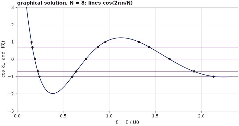
Figure computed by the notebook with open-nemo

Intersections exist only where \(f\) lies between −1 and 1. Every band holds \(N = 8\) states: the lines at \(\cos kL = \pm 1\) (\(k = 0\) and \(k = -\pi/L\)) cross once each per band, and the other six lines are doubly counted because \(+k\) and \(-k\) give the same cosine. Where \(|f| > 1\) there is no intersection for any \(N\): a gap.

2. The band diagram#

Turning the figure by 90° and plotting each intersection at its \(k\) gives the band diagram \(E(k)\). With large \(N\) the points merge into continuous curves. Two common ways to draw them are the reduced zone, all bands folded into \(-\pi/L \le k \le \pi/L\), and the extended zone, band \(j\) placed in \((j-1)\pi/L \le |k| \le j\pi/L\). In the extended zone the bands follow the free-electron parabola \(\hbar^2k^2/2m\) and break away from it at \(k = j\pi/L\), where the gaps open.

open-nemo computes the same bands from the discretized Hamiltonian of one cell (nemo.lead_bands), and the 8-cell intersections are compared with it.

Code56 lines · cell 5

DX = 0.05


def cell_lead(m=M, a=A, b=B, U=U0, dx=DX):
    cell = nemo.Heterostructure1D(
        [nemo.Layer(EM("well", m, 12.9), a), nemo.Layer(EM("barrier", m, 12.9, conduction_band_edge=U), b)],
        spacing=dx,
    )
    h = cell.hamiltonian.sparse.dense().real
    V = np.zeros_like(h)
    V[-1, 0] = -H2M0 / (m * dx**2)
    return nemo.Lead(h, V)


lead = cell_lead()
nemo_states = np.sort(np.concatenate([lead.bands(np.array([2 * np.pi * j / N]))[0][:3] for j in n]))
print(
    f"largest |intersection − open-nemo eigenvalue| for the {len(states)} states: "
    f"{1e3 * np.abs(states - nemo_states[: len(states)]).max():.2f} meV"
)

kL = np.linspace(-np.pi, np.pi, 401)
Ek = np.array([lead.bands(np.array([q]))[0][:4] for q in kL])
fig, (a1, a2) = plt.subplots(1, 2, figsize=(11, 4.5), sharey=True)
for j in range(4):
    a1.plot(kL / np.pi, Ek[:, j], color=style.OPEN_NEMO)
    # extended zone: band j (from 0) occupies j·π/L ≤ |k| ≤ (j+1)·π/L
    kext = j + np.abs(kL) / np.pi if j % 2 == 0 else j + 1 - np.abs(kL) / np.pi
    a2.plot(kext, Ek[:, j], color=style.OPEN_NEMO)
    a2.plot(-kext, Ek[:, j], color=style.OPEN_NEMO)
a1.plot(
    2 * np.pi * n / N / np.pi,
    np.array([lead.bands(np.array([2 * np.pi * j / N]))[0][:3] for j in n]),
    "o",
    ms=3.5,
    color=style.REFERENCE,
)
kk = np.linspace(-4, 4, 400)
a2.plot(kk, H2M0 * (kk * np.pi / L) ** 2 / M, "--", color=style.CONTEXT, lw=1, label="free electron ħ²k²/2m")
for ax in (a1, a2):
    ax.axhline(U0, color=style.CONTEXT, lw=0.6, ls=":")
a1.set(
    xlabel="k L / π", ylabel="energy (eV)", ylim=(0, 1.1), xlim=(-1, 1), title="reduced zone (dots: N = 8)"
)
a2.set(xlabel="k L / π", xlim=(-4, 4), title="extended zone")
a2.legend(frameon=False, fontsize=8)
fig.tight_layout()

print(" band   bottom (eV)   top (eV)   width (meV)   gap above (meV)")
tops = [Ek[:, j].max() for j in range(4)]
bottoms = [Ek[:, j].min() for j in range(4)]
for j in range(3):
    print(
        f"  {j + 1}      {bottoms[j]:.4f}      {tops[j]:.4f}      {1e3 * (tops[j] - bottoms[j]):6.1f}"
        f"          {1e3 * (bottoms[j + 1] - tops[j]):6.1f}"
    )

largest |intersection − open-nemo eigenvalue| for the 24 states: 0.26 meV
 band   bottom (eV)   top (eV)   width (meV)   gap above (meV)
  1      0.0617      0.0961        34.5           143.8
  2      0.2399      0.3822       142.4           146.4
  3      0.5286      0.8521       323.5            92.3

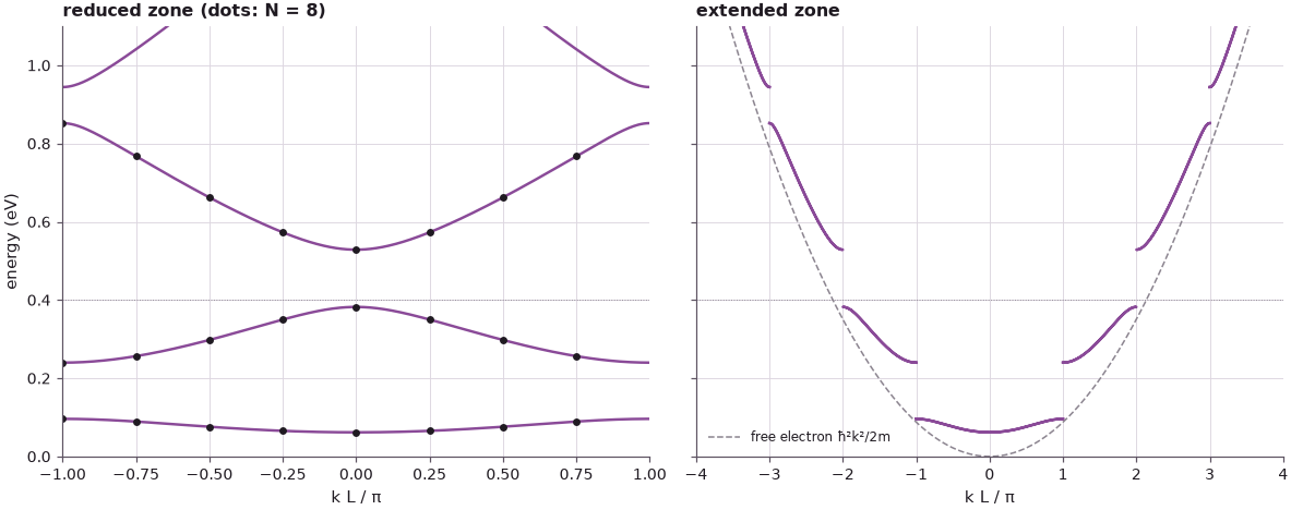
The intersections of the graphical solution and open-nemo's eigenvalues at the same eight \(k\) values agree to the small error of the 0.05 nm grid. In the extended zone the bands hug the free-electron parabola above the barrier top and fall below it in the wells, as a lower average potential requires; at each \(k = j\pi/L\) the curve jumps across a gap. The intersections of the graphical solution agree with open-nemo's eigenvalues to within 0.26 meV. The first gap (0.096 to 0.240 eV, 144 meV) is four times wider than the first band; the second gap (0.382 to 0.529 eV, 146 meV), which straddles the barrier top, is as wide, and the third is narrower (92 meV): far above the barriers the electron feels them less and the gaps shrink.

3. The Brillouin zone and the number of states#

The allowed \(k\) values are spaced by \(\Delta k = 2\pi/(NL)\), and the zone \(-\pi/L \le k < \pi/L\) has width \(2\pi/L\). The number of states per band is therefore

\frac{k_\mathrm{max} - k_\mathrm{min}}{\Delta k} = \frac{2\pi/L}{2\pi/(NL)} = N,

independent of the shape of the band. Klimeck's example: four states per atom and \(N\) atoms give four bands with \(N\) states each. (A factor two for spin is added when electrons are counted.)

Slide 5: Brillouin zone and number of states — Slide 5: the discrete \(k\) points of the ring, \(\Delta k = 2\pi/(NL)\), and \(N\) states per band.

The count is checked on rings of \(N\) cells built from open-nemo's cell Hamiltonian, without using Bloch's theorem: the eigenvalues of the whole ring are sorted into the energy windows of the bands. A coarser grid (0.1 nm) keeps the matrices small.

Code13 lines · cell 7

lead_c = cell_lead(dx=0.1)
h, V = lead_c.h0, lead_c.h1
edges = [(bottoms[j] - 0.01, tops[j] + 0.01) for j in range(3)]
print("  N cells   ring sites   states in band 1   band 2   band 3")
for Nr in (4, 8, 16, 32):
    S = np.roll(np.eye(Nr), 1, axis=1)
    H = np.kron(np.eye(Nr), h) + np.kron(S, V) + np.kron(S.T, V.T)
    ev = np.linalg.eigvalsh(H)
    counts = [int(np.sum((ev > lo) & (ev < hi))) for lo, hi in edges]
    print(
        f"    {Nr:3d}       {H.shape[0]:5d}            {counts[0]:3d}           {counts[1]:3d}      "
        f"{counts[2]:3d}"
    )

  N cells   ring sites   states in band 1   band 2   band 3
      4         320              4             4        4
      8         640              8             8        8
     16        1280             16            16       16
     32        2560             32            32       32

Every band of an \(N\)-cell ring holds exactly \(N\) states, for every \(N\). As \(N\) grows the states fill the band more densely but never spill into the gaps: the band edges are fixed by the cell, the number of states by the size of the crystal.

4. Finite superlattices against the periodic potential#

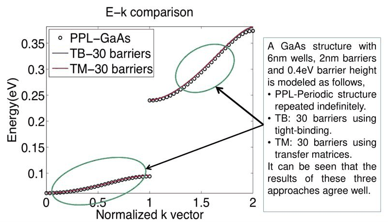
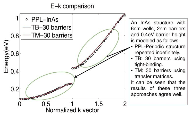
The lecture closes the loop with Section 6. For the GaAs superlattice it compares three calculations: the periodic model of the Periodic Potential Lab (PPL), and the transmission resonances of finite structures with 30 and 80 barriers computed in PCPBT with tight binding (TB) and with transfer matrices (TM). The resonance energies are placed on a normalized \(k\) axis and fall on the periodic bands. The same comparison follows here with open-nemo's transmission (a discretized, tight-binding-like Hamiltonian, as in PCPBT) and an analytic transfer matrix. Lecture 6.4 showed why the resonances can be placed on the \(k\) axis: for \(N_b\) identical barriers, with wells and contacts of the same material, the transmission is exactly one at

q_jL = \frac{j\pi}{N_b}, \qquad j = 1, \dots, N_b - 1 .

Slide 6: GaAs, 30 barriers: PPL, tight binding and transfer matrices — Slide 6: GaAs, 6 nm wells, 2 nm barriers, 0.4 eV: the periodic model (circles) and 30-barrier tight-binding and transfer-matrix results (lines), on a normalized (extended-zone) \(k\) axis.

Code82 lines · cell 9

from scipy.signal import find_peaks


def superlattice(Nb, m=M, dx=DX, lead_len=10.0):
    """Nb barriers (B wide, U0 tall) separated by Nb - 1 wells (A wide), contacts of well material."""
    w_mat, b_mat = EM("well", m, 12.9), EM("barrier", m, 12.9, conduction_band_edge=U0)
    layers = [nemo.Layer(w_mat, lead_len)]
    for j in range(Nb):
        layers.append(nemo.Layer(b_mat, B))
        layers.append(nemo.Layer(w_mat, A if j < Nb - 1 else lead_len))
    return nemo.Heterostructure1D(layers, spacing=dx)


def tmm_T(E, Nb, m=M):
    """Analytic transfer matrix (ψ, ψ') through Nb barriers; contacts of well material at 0 eV."""
    al, be = np.sqrt(m * E / H2M0 + 0j), np.sqrt(m * (E - U0) / H2M0 + 0j)

    def layer(q, d):
        c, s = np.cos(q * d), np.sin(q * d)
        return np.moveaxis(np.array([[c, s / q], [-q * s, c]]), (0, 1), (-2, -1))

    P = layer(be, B)
    total = P.copy()
    cell = P @ layer(al, A)
    for _ in range(Nb - 1):
        total = cell @ total  # (ψ, ψ') on the right = total · (ψ, ψ') on the left
    # incident e^{iαx} + r e^{-iαx} on the left, t e^{iαx} on the right: solve for t
    m11, m12, m21, m22 = total[..., 0, 0], total[..., 0, 1], total[..., 1, 0], total[..., 1, 1]
    t = 2j * al / (1j * al * m11 - m21 + al**2 * m12 + 1j * al * m22)
    return np.abs(t) ** 2


def peak_energies(T, E):
    p = find_peaks(T, height=0.5)[0]
    return E[p]


def band_grid(lo, hi, n=20000, pad=2e-5):
    """Energies dense near the band edges: uniform in q for a cosine band, E = mid − (W/2) cos θ."""
    th = np.linspace(0, np.pi, n)
    return np.r_[lo - pad, 0.5 * (lo + hi) - 0.5 * (hi - lo) * np.cos(th), hi + pad]


def kp_edges(m=M, emax=0.39):
    """Band edges (eV) of the analytic Kronig–Penney model below emax: pairs (bottom, top)."""
    Eg = np.linspace(1e-4, emax, 20000)
    s_ = np.sign(np.abs(kp_f(Eg, m=m)) - 1)
    x = [brentq(lambda e: abs(kp_f(e, m=m)) - 1, Eg[i], Eg[i + 1]) for i in np.nonzero(s_[:-1] != s_[1:])[0]]
    return [(x[i], x[i + 1]) for i in range(0, len(x) - 1, 2)]


def nemo_edges(m=M, nb=2):
    """Band edges of open-nemo's discretized cell (the same grid as the device), from k = 0 and π/L."""
    e0, epi = (cell_lead(m=m).bands(np.array([q]))[0][:nb] for q in (0.0, np.pi))
    return [(min(x, y), max(x, y)) for x, y in zip(e0, epi)]


def kp_energy(q, lo, hi, m=M):
    """Kronig–Penney energy in band (lo, hi) at Bloch wave number q (q L in radians)."""
    return np.array([brentq(lambda e: kp_f(e, m=m) - np.cos(qq), lo, hi) for qq in q])


results = {}
for Nb in (30, 80):
    dev_h = superlattice(Nb).hamiltonian
    counts, dmax, dkp = [], 0.0, 0.0
    for (lo_n, hi_n), (lo_k, hi_k) in zip(nemo_edges(), kp_edges()):
        En, Ek_ = band_grid(lo_n, hi_n), band_grid(lo_k, hi_k)
        e_n = peak_energies(nemo.Transport(dev_h).transmission(En), En)
        e_t = peak_energies(tmm_T(Ek_, Nb), Ek_)
        e_q = np.sort(kp_energy(np.arange(1, Nb) * np.pi / Nb, lo_k, hi_k))  # predicted: q_j L = jπ/Nb
        counts.append((len(e_n), len(e_t)))
        results.setdefault(Nb, []).append(e_n)
        if len(e_t) == len(e_q):
            dkp = max(dkp, np.abs(np.sort(e_t) - e_q).max())
        if len(e_n) == len(e_t):
            dmax = max(dmax, np.abs(e_n - e_t).max())
    print(f"{Nb} barriers: peaks per band (open-nemo, transfer matrix) = {counts}, expected {Nb - 1} each")
    print(
        f"   largest |E transfer matrix − E_KP(q_j)| = {1e3 * dkp:.1e} meV;"
        f"  largest |E open-nemo − E transfer matrix| = {1e3 * dmax:.3f} meV"
    )

30 barriers: peaks per band (open-nemo, transfer matrix) = [(29, 29), (29, 29)], expected 29 each
   largest |E transfer matrix − E_KP(q_j)| = 5.1e-03 meV;  largest |E open-nemo − E transfer matrix| = 0.067 meV
80 barriers: peaks per band (open-nemo, transfer matrix) = [(79, 79), (79, 79)], expected 79 each
   largest |E transfer matrix − E_KP(q_j)| = 5.1e-03 meV;  largest |E open-nemo − E transfer matrix| = 0.067 meV

Both methods find \(N_b - 1\) resonances in each of the two bands below the barrier top, for 30 and for 80 barriers. (The resonances next to a band edge are spaced by only about 0.01 meV for 80 barriers, so the energy grid is made dense near the edges, uniform in \(q\).) The transfer-matrix resonances lie on the Kronig–Penney band at \(q_jL = j\pi/N_b\) to within 0.005 meV (the resolution of the energy grid), and open-nemo's differ from them by at most 0.067 meV, the discretization error of open-nemo's 0.05 nm grid (PCPBT's tight-binding and transfer-matrix curves differ for the same reason). The figure places them on the normalized \(k\) axis, together with the periodic bands from the Kronig–Penney equation.

Code58 lines · cell 11

def kp_bands_extended(m=M, emax=1.1, npts=40000):
    """Energies and extended-zone k L/π from cos kL = f(E): band j in [j-1, j]."""
    Eg = np.linspace(1e-4, emax, npts)
    fg = kp_f(Eg, m=m)
    ok = np.abs(fg) <= 1
    kred = np.arccos(np.clip(fg, -1, 1)) / np.pi  # 0..1 within each band
    band = np.cumsum(np.r_[0, np.diff(ok.astype(int)) == 1]) - (0 if ok[0] else 1)
    kext = np.where(band % 2 == 0, band + kred, band + 1 - kred)
    return Eg[ok], kext[ok]


fig, axes = plt.subplots(1, 3, figsize=(13, 4.2))
for ax, (m, Nb, label) in zip(
    axes, ((M, 30, "GaAs, 30 barriers"), (M, 80, "GaAs, 80 barriers"), (0.023, 30, "InAs, 30 barriers"))
):
    emax = 1.15 if m < 0.05 else 0.39
    Ep, kp = kp_bands_extended(m=m)
    ax.plot(
        kp,
        Ep,
        "o",
        ms=2.5,
        mfc="none",
        color=style.REFERENCE,
        alpha=0.4,
        markevery=max(1, len(Ep) // 70),
        label="periodic (Kronig–Penney)",
    )
    if m == M:
        peaks = results[Nb]  # computed above, band by band
    else:
        dev_h = superlattice(Nb, m=m).hamiltonian
        nb = len(kp_edges(m=m, emax=emax))
        peaks = [
            peak_energies(nemo.Transport(dev_h).transmission(g), g)
            for g in (band_grid(lo, hi, n=6000) for lo, hi in nemo_edges(m=m, nb=nb))
        ]
    for bnd, e in enumerate(peaks):
        # the j-th peak from the bottom of band bnd + 1 sits at |k| L/π = bnd + j/Nb (extended zone)
        ax.plot(
            bnd + np.arange(1, len(e) + 1) / Nb,
            e,
            "-",
            lw=1.0,
            color=style.OPEN_NEMO,
            label="open-nemo transmission peaks" if bnd == 0 else None,
        )
    print(f"{label}: open-nemo peaks per band = {[len(e) for e in peaks]} (expected {Nb - 1})")
    ax.axhline(U0, color=style.CONTEXT, lw=0.6, ls=":")
    ax.set(
        xlabel="normalized k (k L / π, extended zone)",
        ylabel="energy (eV)",
        xlim=(0, len(peaks)),
        ylim=(0, emax),
        title=label,
    )
    ax.legend(frameon=False, fontsize=7, loc="upper left")
fig.tight_layout();

GaAs, 30 barriers: open-nemo peaks per band = [29, 29] (expected 29)
GaAs, 80 barriers: open-nemo peaks per band = [79, 79] (expected 79)
InAs, 30 barriers: open-nemo peaks per band = [29, 29] (expected 29)

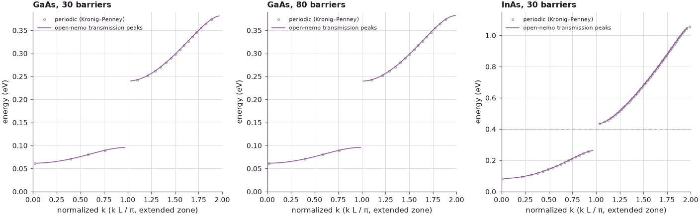
For GaAs with 30 and with 80 barriers, and for InAs (effective mass \(0.023\,m_0\)) with 30 barriers, the transmission resonances of the finite structures lie on the bands of the periodic model, as in the lecture's slides 6 to 8. Going from 30 to 80 barriers only "fills in more dots onto this quasi-continuous line". With the lighter InAs mass the bands move up and widen: the first band spans 0.084 to 0.265 eV, and the second (0.432 to 1.056 eV) lies entirely above the barrier top and is more than 0.6 eV wide, as on slide 8.

Slide 8: InAs, 30 barriers — Slide 8: the same comparison for InAs wells; the lighter mass gives higher and wider bands.

The two pictures, a finite stack probed by transmission and an infinite crystal described by Bloch's theorem, are different approximations to a large but finite solid. Each needs an artificial number, the number of barriers or the number of cells in the ring, and both converge to the same bands.

5. Exploration: weak barriers and the origin of the gaps#

For a weak periodic potential the gaps can be estimated without solving the Kronig–Penney equation. A free electron with \(k = j\pi/L\) and one with \(k = -j\pi/L\) have the same energy, and the Fourier component \(U_j\) of the potential with wave number \(2\pi j/L\) couples them; the degeneracy splits into a gap of width \(2|U_j|\) (the nearly-free-electron result). For barriers of width \(b\) in a period \(L\),

|U_j| = \frac{1}{L}\left|\int_{\mathrm{cell}} U(x)e^{-i2\pi jx/L}dx\right| = \frac{U_0}{j\pi}\left|\sin\frac{j\pi b}{L}\right|.

With \(b/L = 1/4\) the fourth gap should vanish. The gaps from the Kronig–Penney equation are compared with \(2|U_j|\) for \(U_0 = 0.02\) eV.

Code18 lines · cell 13

U_weak = 0.02
Ew = np.linspace(1e-4, 2.6, 520000)
fw = kp_f(Ew, U=U_weak)
ok = np.abs(fw) <= 1
starts = np.nonzero(np.diff(ok.astype(int)) == -1)[0]  # band top: allowed → forbidden
ends = np.nonzero(np.diff(ok.astype(int)) == 1)[0]  # band bottom: forbidden → allowed
ends = ends[ends > starts[0]]  # pair each band top with the next band bottom
print(f"U0 = {1e3 * U_weak:.0f} meV, a = {A} nm, b = {B} nm")
print("  gap j   centre (eV)   width Kronig–Penney (meV)   2|U_j| (meV)")
for j in range(1, 6):
    if j - 1 < len(starts) and j - 1 < len(ends):
        lo, hi = Ew[starts[j - 1]], Ew[ends[j - 1] + 1]
        width = hi - lo
    else:
        lo = hi = np.nan
        width = 0.0
    est = 2 * U_weak / (j * np.pi) * abs(np.sin(j * np.pi * B / L))
    print(f"    {j}      {0.5 * (lo + hi):8.4f}          {1e3 * width:8.3f}              {1e3 * est:7.3f}")

U0 = 20 meV, a = 6.0 nm, b = 2.0 nm
  gap j   centre (eV)   width Kronig–Penney (meV)   2|U_j| (meV)
    1        0.0926             8.915                9.003
    2        0.3558             6.460                6.366
    3        0.7943             3.095                3.001
    4        1.4081             0.055                0.000
    5        2.1973             1.785                1.801

The first three gaps agree with \(2|U_j|\) to within a few per cent, and the fourth gap, where \(\sin(4\pi b/L) = 0\), almost disappears: 0.055 meV instead of several meV, a remainder of second order in \(U_0\) that the first-order estimate ignores. The fifth gap is again open. The gaps are a Bragg effect of the periodic potential, set by its Fourier components, not by the barriers' ability to confine. (For stronger barriers, such as the 0.4 eV of the main example, this estimate no longer holds and the full equation is needed.)

Summary#

\(\cos kL = f(\xi)\) is solved graphically by intersecting \(N\) flat lines with the damped oscillation \(f(\xi)\); intersections exist only where \(|f| \le 1\), giving bands and gaps.
Plotting each intersection at its \(k\) gives the band diagram \(E(k)\), in the reduced zone \([-\pi/L, \pi/L]\) or the extended zone; gaps open at \(k = j\pi/L\).
The \(k\) spacing is \(2\pi/(NL)\), and every band holds exactly \(N\) states.
Finite superlattices of 30 or 80 barriers, computed by transmission (open-nemo or transfer matrices), have resonances that lie on the periodic bands at \(q_jL = j\pi/N_b\).
For weak barriers the gap \(j\) is \(2|U_j|\), twice the Fourier component of the potential.

Exercises#

Repeat the graphical solution with \(N = 5\). How many intersections does each band have, and which line is not doubly counted?
Change the barrier width to \(b = 4\) nm (period 10 nm) and predict which gap vanishes for weak barriers. Check with the code of Section 5.
Plot the ratio of the first band width to the first gap width as a function of \(U_0\) between 0.05 and 1 eV. At which \(U_0\) is the band narrower than 1 meV?
In Section 4, count how many of the 80-barrier transmission peaks of open-nemo lie within 0.1 meV of the Kronig–Penney band computed at \(q_jL = j\pi/80\).