

Lecture 8
Nano-scaled electronic states — basis states, bonding and antibonding
In the lecture
- Why look at the states of a finite multi-well structure, after bands were obtained from transmission peaks: the student questions about Bloch states, bonding and antibonding, and what a band means in a finite system.
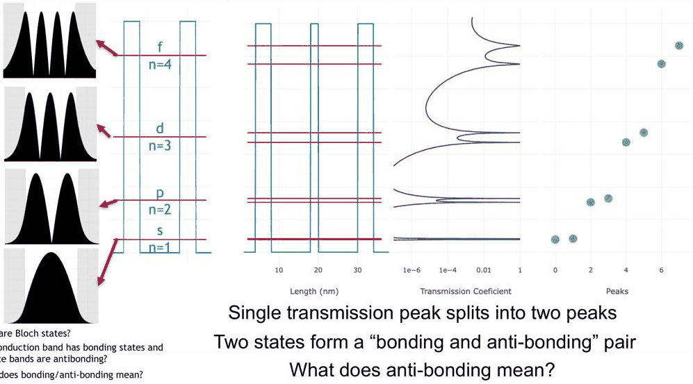
- One quantum well as a "man-made atom": its s-, p-, d- and f-like states, counted by their peaks and zeros.
- Energy-dependent tunnelling: higher states reach further into the barriers.
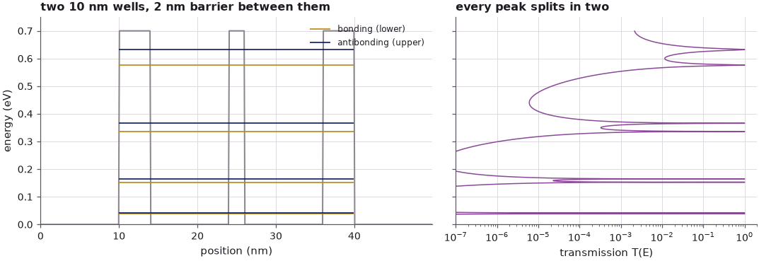
- Two coupled wells: every level splits into a bonding (s + s) and an antibonding (s − s) pair, and the same for the p-, d- and f-like states.
- The basis-state concept: two states interact through an integral ⟨ψ₁|H|ψ₂⟩ and form new states, and the interaction, hence the splitting, grows with energy.
In this notebook
you compute, with open-nemo's effective-mass model of the lecture's PCPBT structures (GaAs wells, 0.7 eV barriers, m* = 0.067 m₀): the resonances and |ψ|² of a 10 nm well between 4 nm barriers; the leakage into the barriers against the single-barrier tunnelling formula; what an asymmetric well does (the lecture's exercise); the bonding and antibonding pairs of two wells and their real wave functions; a two-state (LCAO) model built from the single-well states, compared with the exact pairs; and the splitting as a function of the energy and of the width of the barrier between the wells.
Run it on your own machine
The notebook needs open-nemo (Python ≥ 3.10 and a C++20 compiler; BLAS/LAPACK).
git clone https://github.com/denphi/open-nemo.git && cd open-nemo
python3 -m venv .venv && source .venv/bin/activate
pip install -e ".[notebooks]"
jupyter lab From_Atoms_to_Devices/04_nanoscale_electronic_states/08_0_bonding_and_antibonding_states.ipynbCode
import numpy as np
import matplotlib.pyplot as plt
import opennemo as nemo
from opennemo.visualization import style

style.use(notebook=True)
EMM = nemo.structures.materials.EffectiveMassMaterial
H2M0 = nemo.core.units.HBAR2_2M0          # ħ²/2m₀ in eV nm²
M, V0, DX = 0.067, 0.7, 0.1                # effective mass (m₀), barrier height (eV), grid spacing (nm)
WELL, OUTER, INNER, LEAD = 10.0, 4.0, 2.0, 10.0   # well, outer and inner barrier, lead lengths (nm)
NAMES = "spdf"
gaas = EMM("GaAs", M, 12.9)


def barrier_material(height=V0):
    return EMM(f"barrier {height:g} eV", M, 12.9, conduction_band_edge=height)


def layers(widths, heights=None):
    # alternating barrier, well, barrier, ... of the given widths (nm); `heights` per barrier (eV)
    heights = heights or [V0] * ((len(widths) + 1) // 2)
    return [nemo.Layer(barrier_material(heights[i // 2]) if i % 2 == 0 else gaas, w)
            for i, w in enumerate(widths)]


def open_device(widths, heights=None):
    # the structure between two semi-infinite GaAs leads: a transport problem (PCPBT's view)
    lead = nemo.Layer(gaas, LEAD)
    return nemo.Heterostructure1D([lead] + layers(widths, heights) + [lead], spacing=DX)


def closed_box(widths, heights=None, emax=V0):
    # the same layers with hard walls just outside: real wave functions, energies below `emax`
    box = nemo.Heterostructure1D(layers(widths, heights), spacing=DX)
    sol = nemo.eigenstates(box.hamiltonian.sparse, num=12)
    keep = sol["energies"] < emax
    psi = sol["vectors"][:, keep].real.T
    psi /= np.sqrt((psi**2).sum(axis=1, keepdims=True))   # unit norm on the grid
    for p in psi:                                          # sign: the leftmost lobe positive
        p *= np.sign(p[np.argmax(np.abs(p) > 0.5 * np.abs(p).max())])
    return box, sol["energies"][keep], psi


def decay_length(e, height=V0):
    # 1/κ in the barrier, κ = √(2m(V₀ − E))/ħ (nm)
    return 1 / np.sqrt(M * (height - e) / H2M0)
1. From transmission peaks to the states in a box#
The previous lectures obtained band structure from transport. A structure of N barriers has N − 1 wells, each quasi-bound level of a single well gives N − 1 transmission resonances, the degeneracy of the identical wells is lifted by their interaction, and as N grows the resonances fill cosine-like bands; the lower bands are flatter, so their electrons are heavier. The result is the Kronig–Penney band structure, but obtained in a finite system, which is what real nanostructures are, and without the periodic boundary conditions that Klimeck remembers finding unintuitive as a student ("I can do the math. But wait, what do you mean by included cells?").
Over the years students asked him the questions that drive this lecture and the next: What does band structure mean in a finite system? How many atoms does it take for band structure to emerge? What are Bloch states? What do the textbooks mean when they say that the conduction band has bonding states and the valence band antibonding ones? And what do electronic states "look like" at the nanoscale?
The approach is to forget for a moment that the states were found by computing transport and to look at the structure as a particle in a box. The textbook box with infinite walls, of width \(L\), has the states
on the continuous, convex dispersion \(E(k) = \hbar^2k^2/2m^*\) with \(k = n\pi/L\), and there are infinitely many of them. A real well has barriers of finite height \(V_0\), and only a finite number of states fit below the barrier top. For a symmetric square well of width \(L\) that number is \(\lceil \sqrt{2m^*V_0}\,L/(\pi\hbar)\rceil\):
Code
e_inf = np.arange(1, 7) ** 2 * H2M0 * np.pi**2 / (M * WELL**2)   # infinite walls, L = 10 nm
n_bound = int(np.ceil(np.sqrt(M * V0 / H2M0) * WELL / np.pi))
print("infinite-wall levels of a 10 nm GaAs box (meV):", np.round(e_inf * 1e3, 1))
print(f"states below a {V0} eV barrier top in a {WELL:g} nm well: {n_bound}")
infinite-wall levels of a 10 nm GaAs box (meV): [  56.1  224.5  505.1  898.  1403.1 2020.5]
states below a 0.7 eV barrier top in a 10 nm well: 4
The infinite box would put its fourth level at 898 meV, above the 0.7 eV barriers; the finite well nevertheless holds four states, because leaking into the barriers lowers every level (section 2). The lecture builds its intuition in two steps: one well, then two coupled wells. Lecture 9 then takes the fifteen-well box apart state by state.
2. One quantum well: s-, p-, d- and f-like states#
The single well is the lecture's PCPBT structure: a 10 nm GaAs well between two 4 nm barriers of 0.7 eV,
connected to GaAs leads. The transmission has a sharp peak, reaching 1, at each quasi-bound level, and the
peaks broaden with energy. nemo.resonances returns each level as the complex eigenvalue \(E_0 - i\Gamma/2\)
of the open structure together with its \(|\psi|^2\); \(\Gamma\) is the width of the transmission peak.
Code
dev1 = open_device([OUTER, WELL, OUTER])
res1 = nemo.resonances(dev1)
e = np.unique(np.concatenate([np.linspace(1e-3, V0 - 1e-3, 1500)]
                             + [e0 + w * np.tan(np.linspace(-1.5, 1.5, 81)) / 2
                                for e0, w in zip(res1["energy"], res1["width"])]))
e = e[(e > 0) & (e < V0)]
t1 = nemo.Transport(dev1.hamiltonian).transmission(e)

fig, (a1, a2) = plt.subplots(1, 2, figsize=(10, 3.8), sharey=True, gridspec_kw={"width_ratios": [1.3, 1]})
a1.plot(dev1.x, dev1.band_edge, color=style.CONTEXT, lw=1.3)
a1.hlines(res1["energy"], LEAD, dev1.x[-1] - LEAD, color=style.OPEN_NEMO, lw=1.0)
for n, (e0, rho) in enumerate(zip(res1["energy"], res1["density"])):
    a1.fill_between(dev1.x, e0, e0 + 0.08 * rho / rho.max(), color=style.OPEN_NEMO, alpha=0.4, lw=0)
    a1.text(LEAD - 1, e0, f"{NAMES[n]}, n = {n + 1}", ha="right", va="center", fontsize=8)
a1.set(xlabel="position (nm)", ylabel="energy (eV)", title="10 nm well, 4 nm / 0.7 eV barriers",
       xlim=(0, dev1.x[-1]), ylim=(0, 0.75))
a2.semilogx(t1, e, color=style.OPEN_NEMO, lw=1.0)
a2.set(xlabel="transmission T(E)", xlim=(1e-7, 2), title="transmission")
fig.tight_layout()

print("state  E0 (meV)  E0 / E_n(infinite walls)  width Γ (meV)")
for n, (e0, w) in enumerate(zip(res1["energy"], res1["width"])):
    print(f"{NAMES[n]}, n={n + 1}  {e0 * 1e3:7.1f}   {e0 / e_inf[n]:10.2f}               {w * 1e3:9.4f}")
state  E0 (meV)  E0 / E_n(infinite walls)  width Γ (meV)
s, n=1     40.1         0.72                  0.0040
p, n=2    159.0         0.71                  0.0575
d, n=3    350.4         0.69                  0.5379
f, n=4    596.4         0.66                  5.6784
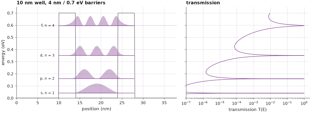
The four levels lie at 40.1, 159.0, 350.4 and 596.4 meV, between 0.72 and 0.66 of the infinite-wall values: the wave function leaks into the barriers, which makes the well effectively wider. Their widths grow by more than three orders of magnitude, from 4.0 μeV for the ground state to 5.7 meV for the fourth: the peaks broaden with energy, as on the lecture's transmission plot.
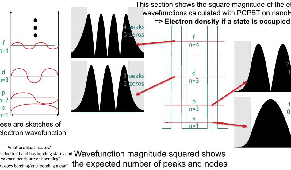
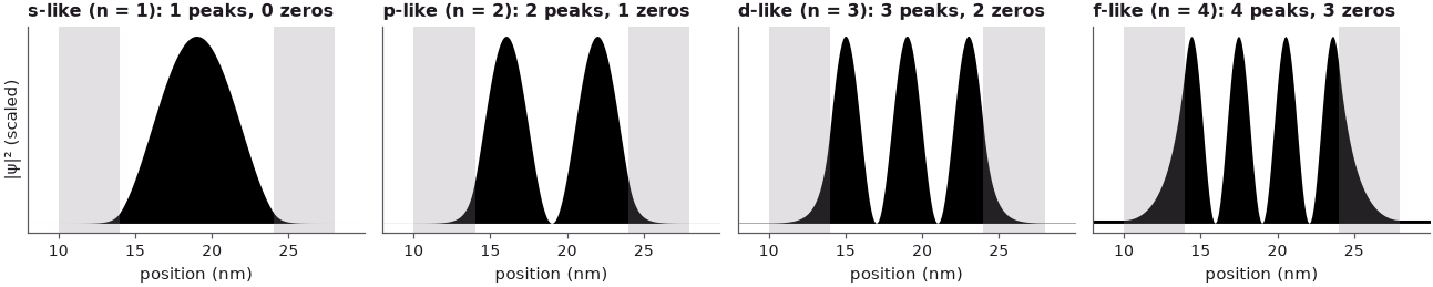
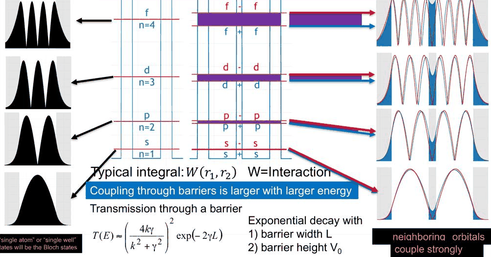
The lecture counts peaks and zeros in |ψ|²: the n-th state has n peaks and n − 1 zeros inside the well. By this count they resemble the s, p, d and f orbitals of an atom, and Klimeck names them so: the well is an artificial atom, and these four states are its basis states. \(|\psi|^2\) is also the electron density the state would carry if it were occupied.
Code
in_well = (dev1.x > LEAD + OUTER) & (dev1.x < LEAD + OUTER + WELL)
in_barrier = dev1.band_edge > V0 / 2
fig, axes = plt.subplots(1, 4, figsize=(12, 2.6), sharey=True)
print("state  peaks  zeros in the well  weight in the barriers  decay length 1/κ (nm)")
for n, (a, e0, rho) in enumerate(zip(axes, res1["energy"], res1["density"])):
    r = rho[in_well]
    peaks = int(np.sum((r[1:-1] > r[:-2]) & (r[1:-1] > r[2:])))
    zeros = int(np.sum((r[1:-1] < r[:-2]) & (r[1:-1] < r[2:])))
    a.fill_between(dev1.x, rho / rho.max(), color="k", lw=0)
    for lo in (LEAD, LEAD + OUTER + WELL):
        a.axvspan(lo, lo + OUTER, color=style.CONTEXT, alpha=0.25, lw=0)
    a.set(xlim=(LEAD - 2, dev1.x[-1] - LEAD + 2), xlabel="position (nm)",
          title=f"{NAMES[n]}-like (n = {n + 1}): {peaks} peaks, {zeros} zeros", yticks=[])
    a.title.set_fontsize(9)
    a.grid(False)
    print(f"{NAMES[n]}, n={n + 1}  {peaks:4d}  {zeros:6d}"
          f"            {rho[in_barrier].sum() / rho.sum():10.1%}"
          f"             {decay_length(e0):10.2f}")
axes[0].set_ylabel("|ψ|² (scaled)")
fig.tight_layout()
state  peaks  zeros in the well  weight in the barriers  decay length 1/κ (nm)
s, n=1     1       0                  0.9%                   0.93
p, n=2     2       1                  3.9%                   1.03
d, n=3     3       2                 10.1%                   1.28
f, n=4     4       3                 23.3%                   2.34
3. Energy-dependent tunnelling into the barriers#
Filling |ψ|² in black, as the lecture does, makes the second point visible: the part of the state inside the barriers grows with energy, from 0.9 % of the s-like state to 23.3 % of the f-like one. Inside a barrier the wave function decays as \(e^{-\kappa x}\) with
so a state closer to the barrier top decays more slowly: the decay length \(1/\kappa\) grows from 0.93 nm to 2.34 nm. The lecture connects this with the tunnelling formula of the previous section for one barrier of width \(L\) (there written with \(\gamma\) for \(\kappa\)):
the thick-barrier limit of the exact result \(T = \left[1 + V_0^2\sinh^2(\kappa L)/(4E(V_0 - E))\right]^{-1}\). The transmission decays exponentially with the barrier width and with the square root of the barrier height above the energy. open-nemo's transmission through one 4 nm barrier, at the four level energies, against both formulas:
Code
single = open_device([OUTER])
t_single = nemo.Transport(single.hamiltonian).transmission(res1["energy"])
print("state  E (meV)   open-nemo T    exact formula   thick-barrier formula")
for n, (e0, t) in enumerate(zip(res1["energy"], t_single)):
    k, kap = np.sqrt(M * e0 / H2M0), np.sqrt(M * (V0 - e0) / H2M0)
    exact = 1 / (1 + V0**2 * np.sinh(kap * OUTER) ** 2 / (4 * e0 * (V0 - e0)))
    approx = (4 * k * kap / (k**2 + kap**2)) ** 2 * np.exp(-2 * kap * OUTER)
    print(f"{NAMES[n]}, n={n + 1}  {e0 * 1e3:6.1f}   {t:.3e}    {exact:.3e}       {approx:.3e}")
state  E (meV)   open-nemo T    exact formula   thick-barrier formula
s, n=1    40.1   1.576e-04    1.565e-04       1.565e-04
p, n=2   159.0   1.152e-03    1.147e-03       1.147e-03
d, n=3   350.4   7.530e-03    7.518e-03       7.546e-03
f, n=4   596.4   6.612e-02    6.623e-02       6.635e-02
The finite-difference transmission agrees with the exact formula to within 0.7 % (the discretization error of the 0.1 nm grid). The thick-barrier formula needs \(\kappa L \gg 1\); \(\kappa L\) is 4.3 for the s-like state and still 1.7 for the f-like one, and the formula stays within 0.2 % of the exact result for all four. From the ground state to the fourth state the transmission of one barrier grows by a factor of about 420, and the resonance widths of section 2 by a factor of 1400: an electron in a higher level escapes faster and, as we shall see, couples more strongly to a neighbouring well.
Klimeck stresses that these real-space states are fixed by their local electrostatic environment: "local potential details specify the details of states with specific symmetries." He leaves an exercise: what happens if the barriers on the left and on the right have different heights or widths? The hint is that more than just the tunnelling should change. Here the right barrier is lowered to 0.5 eV:
Code
asym = open_device([OUTER, WELL, OUTER], heights=[V0, 0.5])
res_a = nemo.resonances(asym)
left_b, right_b = open_device([OUTER]), open_device([OUTER], heights=[0.5])
fig, ax = plt.subplots(figsize=(8, 3.4))
print("state  E0 symmetric  E0 asymmetric (meV)  peak T   4 T_L T_R / (T_L + T_R)²"
      "   weight left : right barrier")
for n, (e0, rho) in enumerate(zip(res_a["energy"], res_a["density"])):
    ee = e0 + res_a["width"][n] * np.linspace(-3, 3, 601)
    t_peak = nemo.Transport(asym.hamiltonian).transmission(ee).max()
    tl = nemo.Transport(left_b.hamiltonian).transmission([e0])[0]
    tr = nemo.Transport(right_b.hamiltonian).transmission([e0])[0]
    wl = rho[(asym.x > LEAD) & (asym.x < LEAD + OUTER)].sum()
    wr = rho[(asym.x > LEAD + OUTER + WELL) & (asym.x < LEAD + 2 * OUTER + WELL)].sum()
    print(f"{NAMES[n]}, n={n + 1}  {res1['energy'][n] * 1e3:8.1f}   {e0 * 1e3:12.1f}        {t_peak:6.3f}"
          f"   {4 * tl * tr / (tl + tr) ** 2:12.3f}             {wl:.4f} : {wr:.4f}")
    ax.plot(asym.x, rho / rho.max() * 0.08 + e0, color=style.sweep(4)[n], lw=1.2)
ax.plot(asym.x, asym.band_edge, color=style.CONTEXT, lw=1.3)
ax.set(xlabel="position (nm)", ylabel="energy (eV)", xlim=(LEAD - 3, asym.x[-1] - LEAD + 3), ylim=(0, 0.75),
       title="asymmetric well: right barrier 0.5 eV (|ψ|² drawn at each level)")
fig.tight_layout()
state  E0 symmetric  E0 asymmetric (meV)  peak T   4 T_L T_R / (T_L + T_R)²   weight left : right barrier
s, n=1      40.1           39.0         0.511          0.511             0.0043 : 0.0073
p, n=2     159.0          154.0         0.482          0.483             0.0182 : 0.0323
d, n=3     350.4          336.8         0.426          0.432             0.0450 : 0.0905
f, n=4     596.4          562.8         0.351          0.409             0.0785 : 0.2159
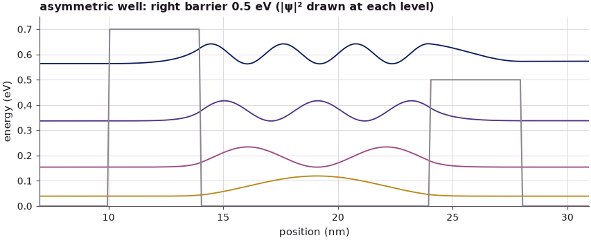
Three things change, not one. The levels move down, by 1.1 meV for the s-like state and 33.6 meV for the f-like one, because the well has become effectively wider on the right; the fourth level, at 562.8 meV, now lies above the 0.5 eV right barrier and is held on that side only by the reflection at the step. The states lose their mirror symmetry: they leak about twice as much into the lower barrier as into the higher one, and the f-like state almost three times as much. And the transmission peaks no longer reach 1: a resonance transmits perfectly only when the electron leaks out to both sides at the same rate. Through a well with barrier transmissions \(T_L\) and \(T_R\), the peak value is \(4T_LT_R/(T_L + T_R)^2\); the computed peaks follow it for the three lower states (0.511, 0.482, 0.426) and fall below it for the fourth (0.351 against 0.409), where the right barrier no longer acts as a tunnelling barrier.
4. Two identical wells: s-like bonding and antibonding#
The lecture now couples two identical quantum systems: two 10 nm wells, kept apart from the leads by 4 nm outer barriers and from each other by a thinner 2 nm barrier, like a molecule of two atoms that are close to each other and isolated from their environment. Every transmission peak of the single well splits into two peaks that both reach 1.
Code
DOUBLE = [OUTER, WELL, INNER, WELL, OUTER]
dev2 = open_device(DOUBLE)
res2 = nemo.resonances(dev2)
e2 = res2["energy"].reshape(4, 2)
e = np.unique(np.concatenate([np.linspace(1e-3, V0 - 1e-3, 1500)]
                             + [e0 + w * np.tan(np.linspace(-1.5, 1.5, 81)) / 2
                                for e0, w in zip(res2["energy"], res2["width"])]))
e = e[(e > 0) & (e < V0)]
t2 = nemo.Transport(dev2.hamiltonian).transmission(e)

fig, (a1, a2) = plt.subplots(1, 2, figsize=(10, 3.6), sharey=True, gridspec_kw={"width_ratios": [1.3, 1]})
a1.plot(dev2.x, dev2.band_edge, color=style.CONTEXT, lw=1.3)
a1.hlines(e2[:, 0], LEAD, dev2.x[-1] - LEAD, color=style.sweep(2)[0], lw=1.1, label="bonding (lower)")
a1.hlines(e2[:, 1], LEAD, dev2.x[-1] - LEAD, color=style.sweep(2)[1], lw=1.1, label="antibonding (upper)")
a1.set(xlabel="position (nm)", ylabel="energy (eV)", title="two 10 nm wells, 2 nm barrier between them",
       ylim=(0, 0.75), xlim=(0, dev2.x[-1]))
a1.legend(frameon=False, fontsize=8, loc="upper right")
a2.semilogx(t2, e, color=style.OPEN_NEMO, lw=1.0)
a2.set(xlabel="transmission T(E)", xlim=(1e-7, 2), title="every peak splits in two")
fig.tight_layout()

print("pair   single well   bonding   antibonding (meV)   splitting (meV)")
for n in range(4):
    print(f"{NAMES[n]}±{NAMES[n]}   {res1['energy'][n] * 1e3:8.2f}"
          f"   {e2[n, 0] * 1e3:8.2f}   {e2[n, 1] * 1e3:8.2f}"
          f"          {(e2[n, 1] - e2[n, 0]) * 1e3:8.3f}")
pair   single well   bonding   antibonding (meV)   splitting (meV)
s±s      40.14      38.66      41.43             2.768
p±p     158.98     152.78     164.67            11.890
d±d     350.36     336.21     365.75            29.541
f±f     596.39     576.06     632.16            56.106
To see the signs of the wave functions, the two wells are closed off: hard walls just outside the 4 nm outer barriers, so the states are real standing waves (the levels move by 0.004 meV for the s-like pair and at most 0.7 meV for the f-like one, printed below). The lower state of the s-like pair is labelled s + s, the upper one s − s; the black curves are the single well's s-like state, copied into the left and into the right well (scaled by 1/√2).
Code
box2, ev2, psi2 = closed_box(DOUBLE)
box1, ev1, psi1 = closed_box([OUTER, WELL, INNER + WELL + OUTER])    # left well alone, same grid
_, _, psi1r = closed_box([OUTER + WELL + INNER, WELL, OUTER])        # right well alone
print("closed box − open structure (meV):", np.round((ev2 - res2["energy"]) * 1e3, 3))


def aligned(psi, ref):
    # the sign that makes ψ agree with the reference state `ref` in the left well
    return psi * np.sign(psi @ ref)


x = box2.x
mid = np.argmin(np.abs(x - x.mean()))                     # centre of the middle barrier
bond, anti = aligned(psi2[0], psi1[0]), aligned(psi2[1], psi1[0])
fig, axes = plt.subplots(1, 2, figsize=(11, 3.3), sharey=True)
for a, sq in zip(axes, (False, True)):
    f = (lambda p: p**2 / (psi2[0] ** 2).max()) if sq else (lambda p: p / np.abs(psi2[0]).max())
    a.fill_between(x, f(bond), color=style.sweep(2)[0], alpha=0.5, lw=0,
                   label=f"s + s, {ev2[0] * 1e3:.2f} meV")
    a.fill_between(x, f(anti), color=style.sweep(2)[1], alpha=0.5, lw=0,
                   label=f"s − s, {ev2[1] * 1e3:.2f} meV")
    for basis in (psi1[0], psi1r[0]):
        a.plot(x, f(basis / np.sqrt(2)), "k", lw=0.9)
    for lo, w in ((0, OUTER), (OUTER + WELL, INNER), (OUTER + 2 * WELL + INNER, OUTER)):
        a.axvspan(lo, lo + w, color=style.CONTEXT, alpha=0.25, lw=0)
    a.axhline(0, color="k", lw=0.5)
    a.set(xlabel="position (nm)", xlim=(0, x[-1]), title="|ψ|²" if sq else "ψ")
    a.grid(False)
axes[0].legend(frameon=False, fontsize=8, loc="lower left")
axes[0].set_ylabel("scaled")
fig.tight_layout()

peak = lambda p: x[np.argmax(np.abs(p) * (x < x.mean()))]  # position of the left-well peak
print(f"|ψ|² at the centre of the middle barrier: bonding {bond[mid] ** 2 / (bond**2).max():.3f}, "
      f"antibonding {anti[mid] ** 2 / (anti**2).max():.1e} (of the peak)")
print(f"left-well peak: single well {peak(psi1[0]):.2f} nm, bonding {peak(bond):.2f} nm, "
      f"antibonding {peak(anti):.2f} nm (middle barrier starts at {OUTER + WELL:.1f} nm)")
print(f"peak-to-peak distance: bonding {2 * (x.mean() - peak(bond)):.2f} nm, "
      f"antibonding {2 * (x.mean() - peak(anti)):.2f} nm")
closed box − open structure (meV): [0.004 0.004 0.023 0.027 0.11  0.145 0.506 0.714]
|ψ|² at the centre of the middle barrier: bonding 0.032, antibonding 6.5e-05 (of the peak)
left-well peak: single well 9.05 nm, bonding 9.15 nm, antibonding 8.95 nm (middle barrier starts at 14.0 nm)
peak-to-peak distance: bonding 11.70 nm, antibonding 12.10 nm
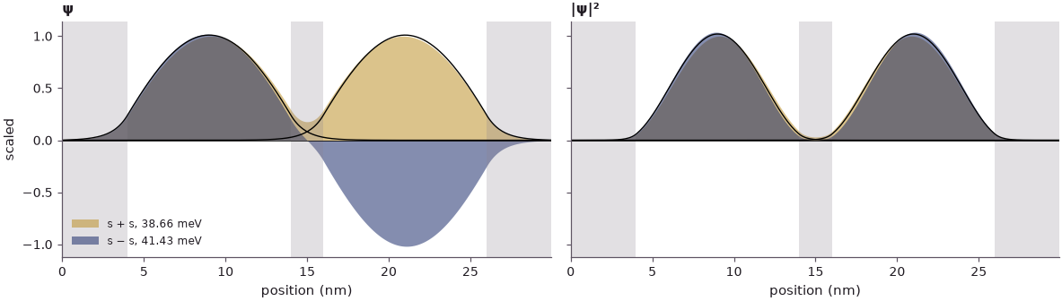
In each well, both states look like the single well's s-like state; the visible difference is in the middle. The lower state has strong overlap in the middle barrier: the two copies of the s-like state are added, and the density at the centre of the barrier is 3.2 % of the peak. The upper state goes through zero at the centre of the barrier: the copies are subtracted, and the density at the centre is 7 × 10⁻⁵ of the peak. Hence the names \(s + s\) and \(s - s\), which Klimeck calls "just nomenclature" but which the black curves justify: the sum and the difference of the single-well states almost coincide with the computed states (section 6 makes this quantitative).
There is more. In the antibonding state the wave function is pushed away from the middle, and its peaks distance themselves from each other. The single well's peak lies at 9.05 nm, the centre of the left well; in the bonding state it moves to 9.15 nm, towards the middle, in the antibonding state to 8.95 nm, away from it, so the two peaks are 11.70 nm apart in the bonding state and 12.10 nm apart in the antibonding one (on the 0.1 nm grid). The shift is small but systematic, and the slides draw it with the same arrows.
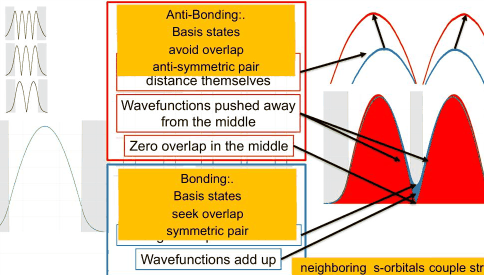
The lecture's summary: in a bonding state the basis states seek overlap, form a symmetric pair and minimize the energy; in an antibonding state they avoid overlap, form an antisymmetric pair and maximize the energy. The extra node in the barrier costs kinetic energy.
5. The p-, d- and f-like pairs#
The same happens one rung up the ladder. The p-like state of the single well has two peaks and one zero, so each state of the p-like pair has two peaks and one zero in each well. The overlap in the middle barrier is even stronger, because the higher state reaches further into the barrier; the antibonding partner again goes to zero there and pushes its peaks outwards. The same holds for the d-like (three peaks per well) and the f-like (four peaks) pairs.
Code
fig, axes = plt.subplots(4, 1, figsize=(10, 7.2), sharex=True)
print("pair   |ψ|² in the middle barrier (share of the state): bonding  antibonding")
mid_b = (x > OUTER + WELL) & (x < OUTER + WELL + INNER)
for n, a in zip(range(4), axes[::-1]):
    b, ab = aligned(psi2[2 * n], psi1[n]), aligned(psi2[2 * n + 1], psi1[n])
    scale = np.abs(b).max()
    a.plot(x, b / scale, color=style.sweep(2)[0], lw=1.4,
           label=f"{NAMES[n]} + {NAMES[n]}, {ev2[2 * n] * 1e3:.1f} meV")
    a.plot(x, ab / scale, color=style.sweep(2)[1], lw=1.4,
           label=f"{NAMES[n]} − {NAMES[n]}, {ev2[2 * n + 1] * 1e3:.1f} meV")
    for lo, w in ((0, OUTER), (OUTER + WELL, INNER), (OUTER + 2 * WELL + INNER, OUTER)):
        a.axvspan(lo, lo + w, color=style.CONTEXT, alpha=0.25, lw=0)
    a.axhline(0, color="k", lw=0.5)
    a.set(yticks=[], ylabel=f"{NAMES[n]}-like pair", xlim=(0, x[-1]))
    a.legend(frameon=False, fontsize=8, loc="upper right", ncol=2)
    a.grid(False)
    print(f"{NAMES[n]}±{NAMES[n]}                                          "
          f"{(b[mid_b] ** 2).sum():.4f}   {(ab[mid_b] ** 2).sum():.1e}")
axes[-1].set_xlabel("position (nm)")
axes[0].set_title("ψ of the four pairs (left-well part drawn with the single-well sign)")
fig.tight_layout()
pair   |ψ|² in the middle barrier (share of the state): bonding  antibonding
s±s                                          0.0078   1.9e-03
p±p                                          0.0321   7.4e-03
d±d                                          0.0734   1.6e-02
f±f                                          0.1215   2.6e-02
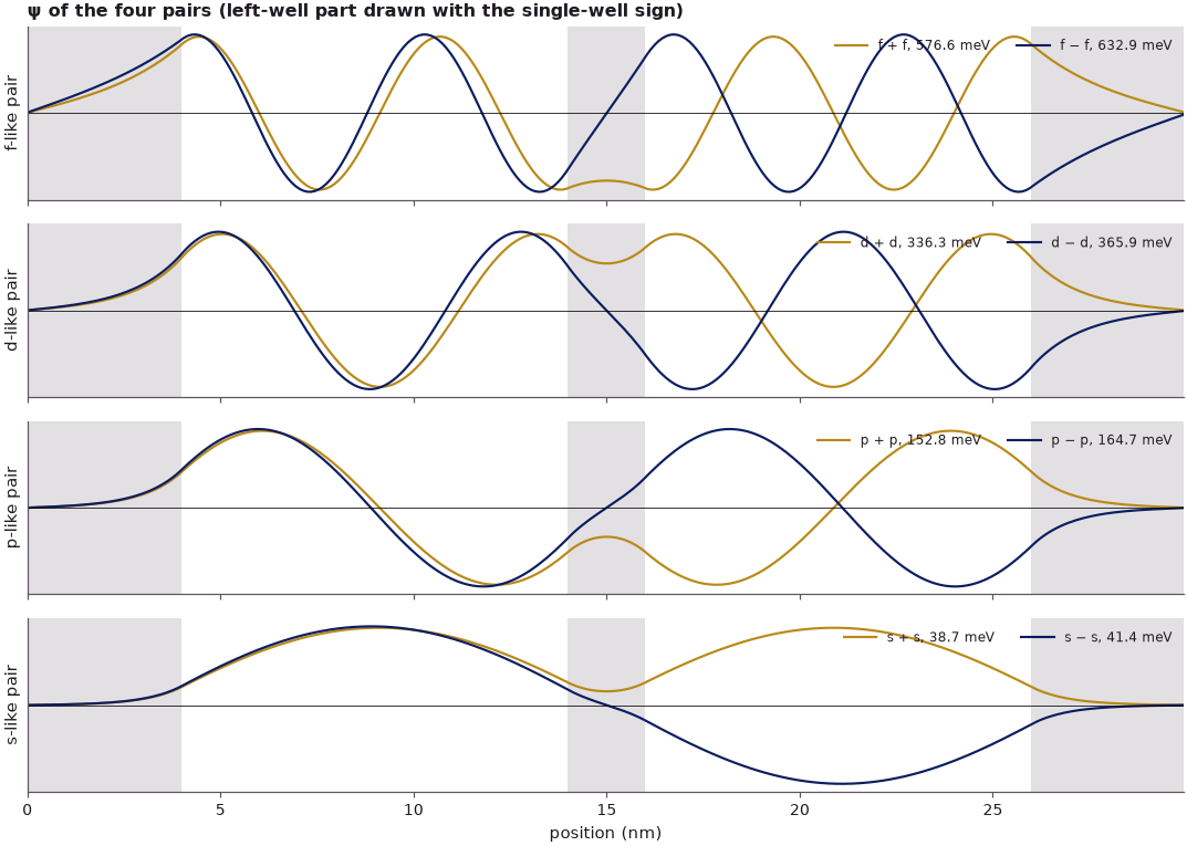
The weight of the bonding state inside the middle barrier grows from 0.8 % (s) to 12.2 % (f); every antibonding state has a node at the centre of the barrier and four to five times less weight in it. The plot of ψ (rather than |ψ|²) shows one rule that the lecture's |ψ|² pictures cannot. For the p- and f-like pairs, which are odd within a well, the right-well part of the bonding state is not a translated copy of the left-well part but its mirror image, which is the translated copy with the sign reversed. What bonds is the agreement of the two lobes that face each other across the middle barrier, not the overall sign. The name "\(p + p\)" refers to the overlap; written with translated copies of one function, the bonding p-like state is a difference. This alternation returns in lecture 9, where it decides which end of a band is bonding.
6. Basis states: two states interact and form new states#
If a single well is like one hydrogen atom, a double well is like an H₂ molecule. The single-well states form a basis set; two of them, \(|\phi_L\rangle\) in the left well and \(|\phi_R\rangle\) in the right one, interact and form new states. Klimeck writes the interaction notionally as ⟨state 1 | interacts | state 2⟩, as an integral
or, in second quantization, \(A = \langle\psi_1|H|\psi_2\rangle\). These "single atom" or "single well" basis states will be the Bloch states of the next lecture. He also notes that one could compute the new states from them by perturbation theory, but that the lecture computes them numerically and uses the basis states for intuition.
Both routes can be compared here. In the basis \(\{\phi_L, \phi_R\}\) the Hamiltonian of the double well is a 2 × 2 matrix with the on-site energy \(\varepsilon = \langle\phi_L|H|\phi_L\rangle\), the interaction \(W = \langle\phi_L|H|\phi_R\rangle\) and the overlap \(S = \langle\phi_L|\phi_R\rangle\) (the basis states are not orthogonal). Its two eigenvalues are
with the eigenvectors \(\phi_L \pm \phi_R\). \(W\) alone depends on the zero of energy when \(S \neq 0\); the combination \(t = W - \varepsilon S\) does not, and the splitting is \(E_+ - E_- = 2|t|/(1 - S^2) \approx 2|t|\). The basis states are the closed single-well states of each well on the same grid, with the other well filled with barrier material (the black curves above); \(\phi_R\) is taken as the mirror image of \(\phi_L\).
Code
h2 = box2.hamiltonian.sparse.dense().real                 # the closed double well's Hamiltonian
print("pair  ε (meV)    t = W − εS (meV)   S        2×2: E(φL+φR) E(φL−φR)"
      "   exact (meV)       |⟨exact|2×2⟩|")
for n in range(4):
    pl, pr = psi1[n], psi1r[n] * np.sign(psi1r[n] @ psi1[n][::-1])   # φR = mirror image of φL
    eps, w, s = pl @ h2 @ pl, pl @ h2 @ pr, pl @ pr
    e_plus, e_minus = (eps + w) / (1 + s), (eps - w) / (1 - s)
    plus, minus = (pl + pr) / np.sqrt(2 + 2 * s), (pl - pr) / np.sqrt(2 - 2 * s)
    fid = [abs(psi2[2 * n] @ plus), abs(psi2[2 * n + 1] @ minus)]   # φL + φR is the lower state
    print(f"{NAMES[n]}    {eps * 1e3:7.2f}   {(w - eps * s) * 1e3:9.3f}        {s:.4f}"
          f"   {e_plus * 1e3:9.2f} {e_minus * 1e3:9.2f}"
          f"     {ev2[2 * n] * 1e3:7.2f} {ev2[2 * n + 1] * 1e3:7.2f}    {fid[0]:.4f} {fid[1]:.4f}")
pair  ε (meV)    t = W − εS (meV)   S        2×2: E(φL+φR) E(φL−φR)   exact (meV)       |⟨exact|2×2⟩|
s      40.11      -1.377        0.0062       38.74     41.49       38.66   41.43    0.9997 0.9998
p     158.74      -5.946        0.0277      152.95    164.85      152.80  164.69    0.9988 0.9990
d     348.94     -14.727        0.0757      335.25    364.87      336.32  365.89    0.9953 0.9947
f     578.19     -21.578        0.1695      559.74    604.18      576.56  632.88    0.9749 0.9543
For the three lower pairs, two basis states and three numbers reproduce the exact states: the energies to within about 1 meV of splittings of 3 to 30 meV, the wave functions with overlaps of 0.995 or better. The hopping \(t\) is negative for all four pairs, so \(\phi_L + \phi_R\) (with \(\phi_R\) the mirror image) is always the lower, bonding state, in agreement with section 5. The f-like pair shows where the picture strains: its basis states overlap by \(S = 0.17\), and close to the barrier top the coupled wells mix in states that the two-state basis does not contain, so the model gives a splitting of about 44 meV instead of 56 meV and overlaps of only 0.97 and 0.95. Klimeck's caveat on the slides, that the interaction strength "W may be energy dependent", is the same observation: a basis built from isolated wells describes the coupling best when it is weak.
7. Why the splitting grows with energy#
The splitting of the pairs grows with energy: 2.77 meV for the s-like pair, 56.1 meV for the f-like one, a factor of 20. The interaction comes from the region where the two basis states overlap, the middle barrier, and each basis state reaches into it with its tail \(e^{-\kappa x}\). The overlap of the two tails across a barrier of width \(b\) scales as \(e^{-\kappa b}\), the square root of the tunnelling probability \(e^{-2\kappa b}\). Coupling through the barriers is larger at larger energy because \(\kappa\) is smaller.
The width of the middle barrier tests this: if the splitting goes as \(e^{-\kappa b}\), its logarithm against \(b\) is a straight line of slope \(-\kappa\), with \(\kappa\) taken at the level energy.
Code
widths = np.arange(1.0, 6.01, 0.5)
split = np.array([np.diff(closed_box([OUTER, WELL, b, WELL, OUTER])[1].reshape(4, 2), axis=1)[:, 0]
                  for b in widths])
fig, ax = plt.subplots(figsize=(7.5, 4))
print("pair   fitted decay constant (1/nm)   κ at the single-well level (1/nm)")
for n in range(4):
    ax.semilogy(widths, split[:, n] * 1e3, "o-", color=style.sweep(4)[n], ms=4, label=f"{NAMES[n]}-like pair")
    slope = -np.polyfit(widths[2:], np.log(split[2:, n]), 1)[0]
    print(f"{NAMES[n]}        {slope:8.3f}                        {1 / decay_length(ev1[n]):8.3f}")
ax.set(xlabel="width of the middle barrier b (nm)", ylabel="splitting E₊ − E₋ (meV)",
       title="splitting against the barrier between the wells")
ax.legend(frameon=False, fontsize=8)
fig.tight_layout()
pair   fitted decay constant (1/nm)   κ at the single-well level (1/nm)
s           1.078                           1.077
p           0.975                           0.975
d           0.783                           0.784
f           0.458                           0.428
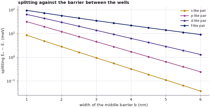
On a logarithmic scale the lines are straight. Fitted from 2 nm upwards, the slopes of the s-, p- and d-like pairs match \(\kappa\) at their levels to 0.1 %; the f-like pair, close to the barrier top, decays 7 % faster than its \(\kappa\) predicts. The splitting falls exponentially with the barrier width, and more slowly the higher the state lies. This is the mechanism behind the observation of lecture 7 that higher bands are wider and lighter: neighbouring wells couple more strongly at higher energy.
Summary#
- A finite well holds a finite number of states (four for 10 nm and 0.7 eV); the n-th has n peaks and n − 1 zeros in |ψ|², and the lecture names them s-, p-, d- and f-like: the well is an artificial atom, its states are its basis set.
- Higher states reach further into the barriers (the barrier weight grows from 0.9 % to 23.3 %), because the decay constant κ = √(2m*(V₀ − E))/ħ falls; the same κ sets the single-barrier transmission and the resonance widths.
- The potential fixes the states: in an asymmetric well the levels shift, the states lose their symmetry and the transmission peaks drop below 1, to 4T_LT_R/(T_L + T_R)².
- Two identical wells turn each level into a pair. The bonding state (lower) has finite density in the middle barrier, the antibonding state (upper) a node there, with its peaks pushed apart.
- A 2 × 2 model in the basis of the two single-well states, with ε, W = ⟨φ_L|H|φ_R⟩ and S, reproduces the s-, p- and d-like pairs; near the barrier top (f-like pair) the isolated-well basis is no longer enough.
- For odd well states (p, f) the bonding partner in the second well is the mirror image, not the translated copy: what bonds is the agreement of the lobes facing each other across the barrier.
- The splitting ≈ 2|t| grows with energy (2.8 to 56 meV here) and falls as e^{−κb} with the barrier width b.
Exercises#
- Give the left and right outer barriers different widths (4 and 6 nm) instead of different heights. Which of the three changes of section 3 survive, and how does the peak transmission compare with 4T_LT_R/(T_L + T_R)²?
- Make the two wells of the double well unequal (10 and 9 nm). Compute the pairs with
closed_box: how much of each state sits in each well, and how does the 2 × 2 model change when the two on-site energies differ? - Repeat section 7 with 0.4 eV barriers. Do the fitted slopes still follow κ, and how many pairs remain?
- Replace the GaAs mass by 0.041 m₀ (an InGaAs-like well). Predict from κ whether the splittings grow or shrink, then check.
Further reading#
- How bands emerge: from one quantum well to fifteen: the same structures carried from one well to fifteen and to the Kronig–Penney bands.
- Benchmark: piecewise-constant barriers against nanoHUB's PCPBT: open-nemo against the tool the lecture's figures come from.
- Quantum transport from scratch: Green's functions on a 1-D chain:
the transmission and the self-energies behind
Transportandresonances. - Tight binding step by step: bonding and antibonding combinations of real atomic orbitals in Si.
- Lecture 9 of this course: the particle in a box revisited.
- nanoHUB tools used on the slides: Piece-Wise Constant Potential Barriers Tool (PCPBT) and the Periodic Potential Lab, nanohub.org.