Lecture 10.7

Introduction to transport — from 1D to 3D: transverse degrees of freedom

In the lecture

a current needs two ingredients, channels and a driving force; the Landauer sum over channels, $I = (2e^2/h)\sum_i T_i\,[f(\mu_L - E) - f(\mu_R - E)]$, is the skeleton of every transport formula
a real RTD is a mesa about 1 µm wide with 5 nm layers, so it is treated as infinitely wide: the wavefunction separates into a plane wave in $x, y$ and a 1-D problem in $z$, and every transverse momentum $\mathbf k_\perp$ (every angle of incidence) is its own channel
$E = E_\perp + E_z$ with $E_\perp = \hbar^2k_\perp^2/2m^*$; $k_\perp$ is conserved across the barriers
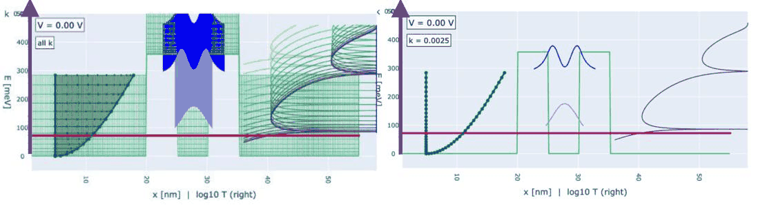
as $k_\perp$ is ramped up, the band edge and the transmission seem to shift up rigidly, while the Fermi level, measured in total energy, stays put
the quantum states and the transmission peaks follow almost perfect parabolas in $k_\perp$, which suggests computing a single transmission at $k_\perp = 0$: the Tsu–Esaki approximation, which Klimeck warns breaks down for most realistic high-performance RTDs

In this notebook

you count the transverse channels of a 1 µm mesa, check that $\mathbf k_\perp$ only shifts $T$ rigidly when the effective mass is the same everywhere, measure how the resonance moves with $k_\perp$ when the barrier is heavier than the well, and compare the full sum over $k_\perp$ with the $k_\perp = 0$ (Tsu–Esaki) current for both cases.

Run the notebookEvery number and figure on this page comes from it. Change it, rerun it, take it further.

Download .ipynb View on GitHub

Run it on your own machine

The notebook needs open-nemo (Python ≥ 3.10 and a C++20 compiler; BLAS/LAPACK).

git clone https://github.com/denphi/open-nemo.git && cd open-nemo
python3 -m venv .venv && source .venv/bin/activate
pip install -e ".[notebooks]"
jupyter lab From_Atoms_to_Devices/05_introduction_to_transport/10_7_transverse_degrees_of_freedom.ipynb

Code11 lines · cell 1

import numpy as np
import matplotlib.pyplot as plt
import opennemo as nemo
from opennemo.visualization import style
from opennemo.structures.statistics import fermi
from opennemo.simulations.analysis import transverse_resolved_current

style.use(notebook=True)
EM = nemo.structures.materials.EffectiveMassMaterial
H2M0, KB = nemo.core.units.HBAR2_2M0, nemo.core.units.KB    # ħ²/2m0 (eV nm²), eV/K
Q, H = nemo.core.units.Q, nemo.core.units.H                 # C, eV s

1. Channels and a driving force#

Lecture 10.3 computed one channel: a plane wave at normal incidence, with transmission $T(E_z)$. In a real device the electrons arrive at every angle. The lecture's picture is a mesa about 1 µm across with 5 nm layers, which for the electrons is an infinite plane.

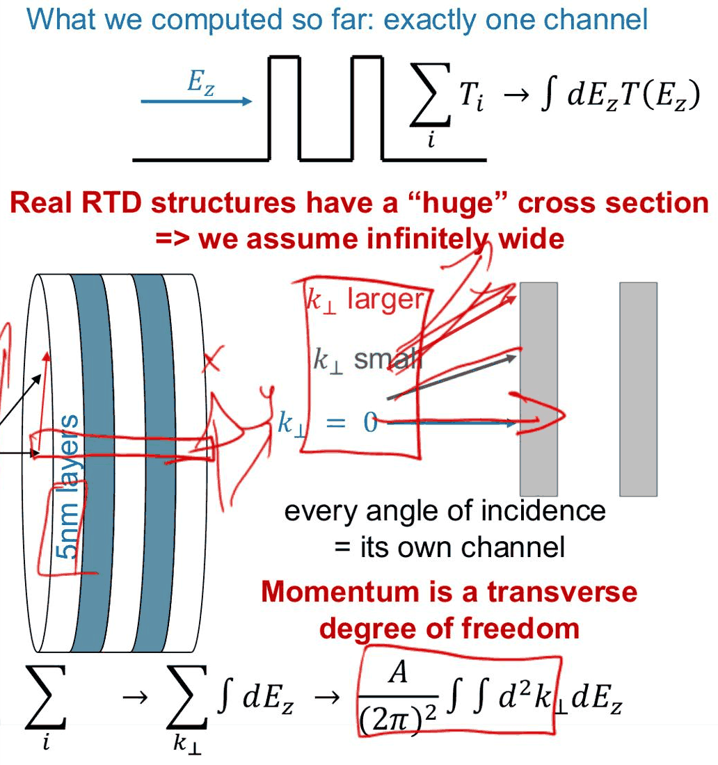
Slide 6: from one channel to many: a 1 µm mesa, transverse momentum as a degree of freedom, and the sum over channels becoming an integral — Slide 6 (with the lecturer's annotations): electrons arriving at $k_\perp = 0$, small $k_\perp$ and larger $k_\perp$ are different channels; the sum over channels becomes $\sum_{k_\perp}\int dE_z \to \frac{A}{(2\pi)^2}\iint d^2k_\perp\,dE_z$.

For a cross section $A$ with periodic boundary conditions the allowed transverse wavevectors sit on a grid of spacing $2\pi/\sqrt A$, one per area $(2\pi)^2/A$ of $k$-space. The number of transverse channels (per spin) with $E_\perp$ below some energy $\epsilon$ is therefore

N(\epsilon) = \frac{A}{(2\pi)^2}\,\pi k_\perp^2 = \frac{A\,m^*\epsilon}{2\pi\hbar^2}.

Code6 lines · cell 3

m_w, side = 0.067, 1000.0             # GaAs mass (m0), mesa side (nm)
for eps in (KB * 4.0, KB * 77.0, KB * 300.0):
    k = np.sqrt(eps * m_w / H2M0)     # 1/nm
    print(f"E_perp < {eps * 1e3:6.2f} meV: k_perp < {k:.3f} /nm, "
          f"{side**2 * k**2 / (4 * np.pi):8.0f} channels per spin in a 1 µm x 1 µm mesa")
print(f"spacing of the transverse k grid: {2 * np.pi / side:.4f} /nm")

E_perp <   0.34 meV: k_perp < 0.025 /nm,       48 channels per spin in a 1 µm x 1 µm mesa
E_perp <   6.64 meV: k_perp < 0.108 /nm,      929 channels per spin in a 1 µm x 1 µm mesa
E_perp <  25.85 meV: k_perp < 0.213 /nm,     3618 channels per spin in a 1 µm x 1 µm mesa
spacing of the transverse k grid: 0.0063 /nm

Within one thermal energy at room temperature there are about 3600 transverse channels per spin, on a $k$ grid with spacing $0.0063$ nm$^{-1}$, much finer than any structure in $T(E, k_\perp)$. That is why the sum over channels can be replaced by an integral, and why the edges of the mesa do not matter.

2. Separation of variables#

With an infinite cross section and a potential that depends only on $z$, the Schrödinger equation separates:

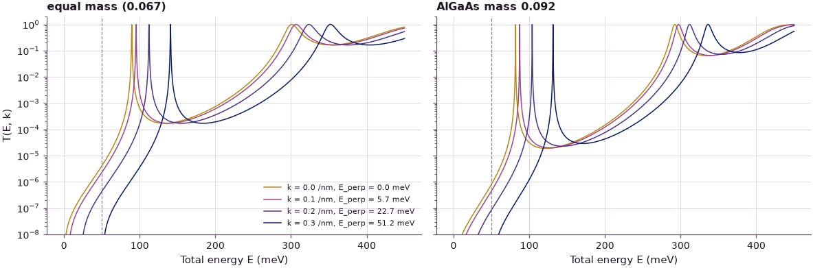
\psi(\mathbf r) = \frac{e^{i\mathbf k_\perp\cdot\mathbf r_\perp}}{\sqrt A}\,\varphi(z),\qquad \left[-\frac{\hbar^2}{2}\frac{d}{dz}\frac{1}{m^*(z)}\frac{d}{dz} + V(z) + \frac{\hbar^2k_\perp^2}{2m^*(z)}\right] \varphi(z) = E\,\varphi(z).

The transverse kinetic energy enters the 1-D problem as an extra potential $\hbar^2k_\perp^2/2m^*(z)$. If the mass is the same everywhere, that potential is a constant $E_\perp$; it shifts the whole 1-D problem rigidly, and $T(E, k_\perp) = T(E - E_\perp, 0)$ exactly, with $E_z = E - E_\perp$ the longitudinal energy. If the barrier is heavier than the well, the barrier rises by less than the well and the shift is no longer rigid.

The device is the double barrier of Lectures 10.1–10.4 (10 nm GaAs, 5 nm AlGaAs, 5 nm GaAs, 5 nm AlGaAs, 10 nm GaAs, a 0.3 eV barrier) in two versions: with the AlGaAs mass set equal to that of GaAs, and with its own mass 0.092 $m_0$. In open-nemo the transverse term is passed to Transport as a potential, H2M0 * k**2 / dev.mass.

Code22 lines · cell 5

gaas = EM("GaAs", m_w, 12.9)


def device(barrier_mass):
    algaas = EM("AlGaAs", barrier_mass, 12.2, conduction_band_edge=0.3)
    layers = [nemo.Layer(m, w) for m, w in ((gaas, 10), (algaas, 5), (gaas, 5), (algaas, 5), (gaas, 10))]
    return nemo.Heterostructure1D(layers, spacing=0.05, mass_average="mean")


devices = {"equal mass (0.067)": device(0.067), "AlGaAs mass 0.092": device(0.092)}
x = devices["equal mass (0.067)"].x
transverse = {name: (lambda k, d=d: H2M0 * k**2 / d.mass) for name, d in devices.items()}

dev = devices["equal mass (0.067)"]
tr = nemo.Transport(dev.hamiltonian)
e = np.linspace(0.06, 0.25, 4001)
for k in (0.1, 0.2, 0.3):
    e_perp = H2M0 * k**2 / m_w
    t_k = tr.transmission(e, potential=transverse["equal mass (0.067)"](k))
    t_shift = tr.transmission(e - e_perp)
    print(f"equal mass, k = {k} /nm: E_perp = {e_perp * 1e3:6.2f} meV, "
          f"max |T(E,k) - T(E - E_perp, 0)| = {np.abs(t_k - t_shift).max():.1e}")

equal mass, k = 0.1 /nm: E_perp =   5.69 meV, max |T(E,k) - T(E - E_perp, 0)| = 1.7e-10
equal mass, k = 0.2 /nm: E_perp =  22.75 meV, max |T(E,k) - T(E - E_perp, 0)| = 5.2e-12
equal mass, k = 0.3 /nm: E_perp =  51.18 meV, max |T(E,k) - T(E - E_perp, 0)| = 1.7e-10

For equal masses the identity holds to round-off: the transverse momentum only relabels the energy.

Slide 33: the band edge and the transmission shift up rigidly with transverse momentum, while the Fermi level stays fixed in total energy — Slide 33: left, the band edge, the states and $\log_{10}T$ for all transverse momenta; right, one frame at $k = 0.0025$ (in Å$^{-1}$). The red line is the Fermi level, fixed in total energy.

The figure below makes the same picture for the two devices: $T$ against total energy for four transverse wavevectors, with the zero-bias Fermi level of 50 meV used in the rest of the notebook.

Code14 lines · cell 7

ks = np.array([0.0, 0.1, 0.2, 0.3])
e = np.linspace(0.0, 0.45, 9001)
mu = 0.05
fig, axes = plt.subplots(1, 2, figsize=(11, 3.8), sharey=True)
for ax, (name, d) in zip(axes, devices.items()):
    trd = nemo.Transport(d.hamiltonian)
    for k, c in zip(ks, style.sweep(len(ks))):
        ax.semilogy(e * 1e3, trd.transmission(e, potential=transverse[name](k)), color=c, lw=1,
                    label=f"k = {k:.1f} /nm, E_perp = {H2M0 * k**2 / m_w * 1e3:.1f} meV")
    ax.axvline(mu * 1e3, color=style.CONTEXT, ls="--", lw=0.8)
    ax.set(xlabel="Total energy E (meV)", title=name, ylim=(1e-8, 2))
axes[0].set_ylabel("T(E, k)")
axes[0].legend(frameon=False, fontsize=7, loc="lower right")
fig.tight_layout()

Figure computed by the notebook with open-nemo

3. How the resonance moves with $k_\perp$#

The emitter injects electrons whose transverse energy is $\hbar^2k_\perp^2/2m_w$ with the GaAs mass. The resonance moves by $\hbar^2k_\perp^2/2m_\parallel$ with an in-plane mass $m_\parallel$ of the quasi-bound state. To first order in $k_\perp^2$ the shift is the expectation value of the transverse term,

\Delta E_r(k_\perp) \approx \frac{\hbar^2k_\perp^2}{2}\left\langle\frac{1}{m^*(z)}\right\rangle = \frac{\hbar^2k_\perp^2}{2}\int\frac{|\varphi(z)|^2}{m^*(z)}\,dz,

so a state with a fraction $P_b$ of its probability in the barriers sees an average of the two masses.

Code18 lines · cell 9

d = devices["AlGaAs mass 0.092"]
r0 = nemo.resonances(d)
rho = r0["density"][0] / np.sum(r0["density"][0])      # |phi|^2 of the lowest state, normalized
in_barrier = d.mass > m_w + 1e-9
inv_mass = np.sum(rho / d.mass)
print(f"lowest state at k = 0: E_r = {r0['energy'][0] * 1e3:.2f} meV, "
      f"probability in the barriers P_b = {rho[in_barrier].sum():.3f}, "
      f"<1/m> = 1/{1 / inv_mass:.4f} m0")
print("\n  k (/nm)  E_perp emitter   shift E_r(k)-E_r(0)   first-order <1/m>   shift / E_perp")
k_line = np.linspace(0.0, 0.8, 17)
shift = {}
for name, dd in devices.items():
    shift[name] = np.array([nemo.resonances(dd, potential=transverse[name](k))["energy"][0]
                            for k in k_line]) - nemo.resonances(dd)["energy"][0]
for k, s in zip(k_line[::4], shift["AlGaAs mass 0.092"][::4]):
    e_perp = H2M0 * k**2 / m_w
    print(f"  {k:5.2f}     {e_perp * 1e3:7.2f} meV       {s * 1e3:7.2f} meV       "
          f"{H2M0 * k**2 * inv_mass * 1e3:7.2f} meV        {s / e_perp if k else 1:.4f}")

lowest state at k = 0: E_r = 81.79 meV, probability in the barriers P_b = 0.111, <1/m> = 1/0.0691 m0

  k (/nm)  E_perp emitter   shift E_r(k)-E_r(0)   first-order <1/m>   shift / E_perp
   0.00        0.00 meV          0.00 meV          0.00 meV        1.0000
   0.20       22.75 meV         22.05 meV         22.06 meV        0.9695
   0.40       90.98 meV         88.12 meV         88.24 meV        0.9686
   0.60      204.72 meV        197.93 meV        198.54 meV        0.9669
   0.80      363.94 meV        350.86 meV        352.96 meV        0.9641

The lowest state has 11% of its probability in the barriers, which gives an in-plane mass of 0.0691 $m_0$ instead of 0.067 $m_0$. Its shift therefore lags behind the emitter parabola, by 3.0% at small $k_\perp$ and by 3.6% at $k_\perp = 0.8$ nm$^{-1}$, where the state is pushed further into the barriers. The first-order estimate from $\langle 1/m\rangle$ at $k_\perp = 0$ is 0.12 meV high at $k_\perp = 0.4$ nm$^{-1}$ and 2.1 meV high at 0.8 nm$^{-1}$.

Slide 37: the band edges, the emitter's 2-D density of states, the confined states and the transmission peaks as functions of energy and transverse momentum — Slide 37: the band edge $E_c(z,k)$, the emitter states (green) and the transmission peaks (blue) as functions of $k$ (0 to 0.07 Å$^{-1}$); right, the projection onto energy and $k$, where the peaks follow parabolas.

The projection on the right of slide 37 is reproduced below for the device with the heavier barrier: the emitter band bottom $E_\perp(k_\perp)$, the lowest resonance and the Fermi level.

Code18 lines · cell 11

fig, (a1, a2) = plt.subplots(1, 2, figsize=(11, 3.8))
a1.plot(k_line, H2M0 * k_line**2 / m_w * 1e3, color=style.CONTEXT, lw=2,
        label="emitter band bottom E_perp(k)")
for (name, s), c in zip(shift.items(), (style.REFERENCE, style.OPEN_NEMO)):
    a1.plot(k_line, (r0["energy"][0] + s) * 1e3, "o-", ms=3, color=c, label=f"lowest resonance, {name}")
a1.axhline(mu * 1e3, color=style.CONTEXT, ls="--", lw=0.8, label="Fermi level (total energy)")
a1.set(xlabel="k_perp (1/nm)", ylabel="Total energy (meV)", title="Parabolas in k_perp")
a1.legend(frameon=False, fontsize=7)
lag = (H2M0 * k_line**2 / m_w - shift["AlGaAs mass 0.092"]) * 1e3
a2.plot(k_line, lag, "o-", ms=3, color=style.OPEN_NEMO, label="AlGaAs mass 0.092")
a2.plot(k_line, (H2M0 * k_line**2 / m_w - shift["equal mass (0.067)"]) * 1e3, "s--", ms=3,
        color=style.REFERENCE, label="equal mass")
a2.set(xlabel="k_perp (1/nm)", ylabel="E_perp(k) − ΔE_r(k) (meV)",
       title="Resonance lag behind the emitter parabola")
a2.legend(frameon=False, fontsize=8)
fig.tight_layout()
print(f"lag at k = 0.4 /nm: {lag[8]:.2f} meV; at 0.8 /nm: {lag[-1]:.2f} meV "
      f"(resonance width {r0['width'][0] * 1e3:.3f} meV)")

lag at k = 0.4 /nm: 2.86 meV; at 0.8 /nm: 13.08 meV (resonance width 0.129 meV)

On the scale of the left panel the parabolas lie almost on top of each other, which is what slide 37 shows: "all transverse momentum behavior looks perfectly parabolic". The right panel shows that the lag is not small compared with the resonance: at $k_\perp = 0.4$ nm$^{-1}$, a transverse energy of 91 meV, the heavy-barrier resonance sits 2.9 meV lower in longitudinal energy than at $k_\perp = 0$, more than 20 times its width of 0.129 meV.

4. Summing all channels: full $k_\perp$ integral versus Tsu–Esaki#

The current density sums the Landauer current of every channel, with the occupation set by the total energy $E$ (two spins, $\int d^2k_\perp/(2\pi)^2 = \int k\,dk/2\pi$):

J = \frac{2e}{h}\int_0^\infty\frac{k\,dk}{2\pi}\int dE\;T(E, k)\,[f(E - \mu_L) - f(E - \mu_R)].

The Tsu–Esaki approximation assumes $T(E, k) = T(E - E_\perp, 0)$ with the emitter mass and does the $k$ integral analytically (Lecture 10.8). dev.current_density evaluates that one-dimensional form. Below, the full integral is computed with 48 Gauss–Legendre points in $k$ and an energy grid adapted to the resonances at each $k$, on the linear-drop potential of Lecture 10.1 (the bias drops across the 15 nm double barrier) with $\mu_L = 50$ meV, $\mu_R = \mu_L - eV$ and $T = 300$ K.

Code42 lines · cell 13

T = 300.0


def linear_drop(v):
    return -v * np.clip((x - 10.0) / 15.0, 0.0, 1.0)


def energy_grid(d, u, lo, hi):
    res = nemo.resonances(d, potential=u)
    parts = [np.linspace(lo, hi, 4000)]
    parts += [er + w * np.linspace(-40, 40, 401)
              for er, w in zip(res["energy"], res["width"]) if lo < er < hi]
    e = np.unique(np.concatenate(parts))
    return e[(e >= lo) & (e <= hi)]


def currents(name, v, num_k=48):
    d, u0 = devices[name], linear_drop(v)
    trd = nemo.Transport(d.hamiltonian)
    lo, hi = -v + 1e-5, mu + 15 * KB * T
    e0 = energy_grid(d, u0, lo, hi)
    j_te = d.current_density(e0, trd.transmission(e0, potential=u0), mu, mu - v, T)
    k_max = np.sqrt((hi - lo) * 0.092 / H2M0)
    xg, wg = np.polynomial.legendre.leggauss(num_k)
    kk, wk = 0.5 * k_max * (xg + 1), 0.5 * k_max * wg
    per_k = []
    for k in kk:
        uk = u0 + transverse[name](k)
        ek = energy_grid(d, uk, lo, hi)
        occ = fermi(ek, mu, T) - fermi(ek, mu - v, T)
        per_k.append(k / np.pi * np.trapezoid(trd.transmission(ek, potential=uk) * occ, ek))
    per_k = Q / H * np.array(per_k) * 1e14            # dJ/dk, A/cm^2 per (1/nm)
    return j_te, float(np.dot(wk, per_k)), kk, per_k


results = {}
print("                        V (V)   Tsu-Esaki (A/cm^2)   full k sum (A/cm^2)   ratio")
for name in devices:
    for v in (0.05, 0.1, 0.15):
        results[name, v] = currents(name, v)
        j_te, j_k = results[name, v][:2]
        print(f"  {name:20s}  {v:.2f}     {j_te:10.1f}          {j_k:10.1f}         {j_k / j_te:.4f}")

                        V (V)   Tsu-Esaki (A/cm^2)   full k sum (A/cm^2)   ratio
  equal mass (0.067)    0.05         6358.1              6355.9         0.9997
  equal mass (0.067)    0.10        11573.0             11578.6         1.0005
  equal mass (0.067)    0.15        11410.3             11389.5         0.9982
  AlGaAs mass 0.092     0.05         2471.1              2904.6         1.1754
  AlGaAs mass 0.092     0.10         4158.2              4912.5         1.1814
  AlGaAs mass 0.092     0.15         3032.6              3239.2         1.0681

With equal masses the two agree to within 0.2%, the accuracy of the $k$ and energy quadratures: here Tsu–Esaki is exact. With the heavier barrier the full sum gives 18% more current at 0.05 and 0.1 V and 7% more at 0.15 V. At every $k_\perp$ the resonance sits slightly lower in longitudinal energy than Tsu–Esaki assumes; the lag is many resonance widths, and at these biases the resonance lies in the energy range where the emitter supply grows towards lower energy, so the lower resonance carries more current.

The library's transverse_resolved_current does the same sum on one energy grid for all $k$. As a cross check, it is given the union of the resonance-adapted grids at its own 32 Gauss–Legendre points.

Code9 lines · cell 15

name, v = "AlGaAs mass 0.092", 0.1
d, u0 = devices[name], linear_drop(v)
lo, hi = -v + 1e-5, mu + 15 * KB * T
k_max = np.sqrt((hi - lo) * 0.092 / H2M0)
nodes = 0.5 * k_max * (np.polynomial.legendre.leggauss(32)[0] + 1)
grid = np.unique(np.concatenate([energy_grid(d, u0 + transverse[name](k), lo, hi) for k in nodes]))
j_lib = transverse_resolved_current(d, grid, mu, mu - v, T, potential=u0, num_k=32, k_max=k_max)
print(f"{name}, V = {v} V: transverse_resolved_current {j_lib:.1f} A/cm^2 on {grid.size} energies, "
      f"notebook sum {results[name, v][1]:.1f} A/cm^2")

AlGaAs mass 0.092, V = 0.1 V: transverse_resolved_current 4912.3 A/cm^2 on 16577 energies, notebook sum 4912.5 A/cm^2

The two agree to 0.01%. The last figure shows where in $k_\perp$ the current comes from at 0.1 V: the integrand $dJ/dk$ of the full sum for both devices, and the Tsu–Esaki integrand, which for the emitter mass is the same function for both devices with $T(E_z)$ taken at $k_\perp = 0$.

Code8 lines · cell 17

fig, ax = plt.subplots(figsize=(6.2, 3.8))
for (name, c) in zip(devices, (style.REFERENCE, style.OPEN_NEMO)):
    j_te, j_k, kk, per_k = results[name, 0.1]
    ax.plot(kk, per_k / 1e3, "o-", ms=3, color=c,
            label=f"{name}: J = {j_k:.0f} A/cm² (Tsu–Esaki {j_te:.0f})")
ax.set(xlabel="k_perp (1/nm)", ylabel="dJ/dk (kA/cm² per 1/nm)",
       title="Current per transverse wavevector, 0.1 V")
ax.legend(frameon=False, fontsize=8);

Both distributions start at zero ($dJ/dk \propto k$, the area of the ring in $k$-space) and fall off when $E_\perp$ exceeds the Fermi level by a few $k_BT$; the bulk of the current comes from $k_\perp \lesssim 0.4$ nm$^{-1}$, where the lag of Section 3 is already several resonance widths.

5. Where the shortcut fails#

Slide 39: the band diagram of a realistic high-performance RTD, where the Tsu–Esaki approximation breaks down — Slide 39: the band edge of a more realistic RTD at $k = 0$ under bias, with deep wells between tall barriers and a strongly sloped collector.

Slide 38 sums up the conclusion of the lecture: because everything looks parabolic, "just calculate ONE transmission at k=0"; no numerical sum over $k$ is needed. Klimeck adds that later sections will show this "breaks down COMPLETELY for most realistic high-performance RTDs". Section 4 shows the mechanism in its mildest form: any difference between the in-plane dispersion of the emitter and that of the resonant state moves the resonance relative to the injected electrons as $k_\perp$ grows. Here a 37% heavier barrier changes the current by up to 18%. In real RTDs the bands are nonparabolic (the mass grows with energy, more in narrow-gap InGaAs and in the barrier materials), the wells are deep and the barriers tall, and the lag grows accordingly. The full $k_\perp$ sum costs one 1-D calculation per transverse wavevector; Lecture 10.8 derives the formula that avoids it, at the price of the assumption tested here.

Summary#

A 1 µm mesa has about 3600 transverse channels per spin within $k_BT$ at 300 K, on a $k$ grid of 0.0063 nm$^{-1}$; the sum over channels becomes an integral over $\mathbf k_\perp$.
Separation of variables puts $\hbar^2k_\perp^2/2m^*(z)$ into the 1-D problem as a potential; with one mass everywhere $T(E, k_\perp) = T(E - E_\perp, 0)$ exactly, while the Fermi level stays fixed in total energy.
With a heavier barrier (0.092 versus 0.067 $m_0$) the lowest resonance has $P_b = 0.11$ and an in-plane mass of 0.0691 $m_0$; at $k_\perp = 0.4$ nm$^{-1}$ it lags the emitter parabola by 2.9 meV, more than 20 resonance widths.
The full $k_\perp$ integral equals the Tsu–Esaki current to 0.2% for equal masses and exceeds it by up to 18% for the heavier barrier; transverse_resolved_current reproduces the notebook's sum to 0.01%.

Exercises#

Repeat Section 4 at 77 K. Does the ratio between the full sum and Tsu–Esaki grow or shrink, and how does that relate to the range of $k_\perp$ that carries the current?
Set the AlGaAs mass to 0.050 $m_0$ (lighter than the well). In which direction does the resonance lag, and how does the ratio change?
Compute the first-order shift $\hbar^2k_\perp^2\langle 1/m\rangle/2$ for the second resonance at 292 meV. Is its in-plane mass closer to that of the barrier, and why?