Course/02 · Materials and quantum mechanics

ECE 606 Lecture 4.3

Why do we need quantum mechanics?

In the lecture

the question of Section 4 once more: the density of electrons available for conduction is not the number of atoms per volume times the electrons per atom
the problem to solve: electrons in the periodic potential of a crystal, pictured as square buckets around the atomic cores
a skier passing obstacles would follow Newton's laws, but electrons can be tightly bound to the cores, loosely bound, or free to move through the structure
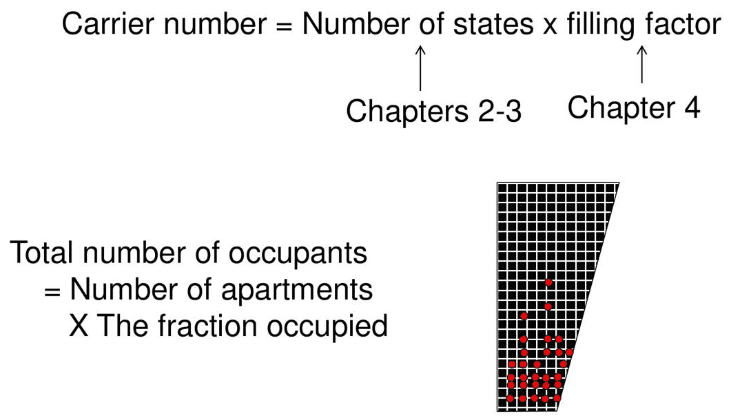
even free electrons need empty states to move into: the carrier number is the number of states times their filling, like the occupants of an apartment building
the outlook: the Schrödinger equation arises from quantization and relativity, and the next lectures solve concrete problems with it

In this notebook

builds the lecture's picture of electrons in square buckets as a one-dimensional Kronig–Penney crystal, computes its bands with open-nemo's periodic-lead solver and checks the band edges against the analytic Kronig–Penney condition, shows that deep bands are narrow and slow (bound electrons) and high bands free-electron-like, and then fills the states with the Fermi function to show that the number of electrons that respond to a field depends on the filling, not on the number of electrons.

Run the notebookEvery number and figure on this page comes from it. Change it, rerun it, take it further.

Download .ipynb View on GitHub

Run it on your own machine

The notebook needs open-nemo (Python ≥ 3.10 and a C++20 compiler; BLAS/LAPACK).

git clone https://github.com/denphi/open-nemo.git && cd open-nemo
python3 -m venv .venv && source .venv/bin/activate
pip install -e ".[notebooks]"
jupyter lab From_Atoms_to_Devices/02_materials_and_quantum_mechanics/04_3_why_quantum_mechanics.ipynb

Code9 lines · cell 1

import numpy as np
import matplotlib.pyplot as plt
import opennemo as nemo
from opennemo.visualization import style

style.use(notebook=True)
from opennemo.core.units import HBAR, HBAR2_2M0, KB, M0, Q
from scipy.optimize import brentq
from scipy.special import expit

1. The problem: electrons in a periodic potential#

The current needs the density \(n\) of electrons that can move, and Lectures 3.1 and 4.1 showed that \(n \neq N\times\rho\): not every electron of the crystal conducts. Klimeck now zooms into the device. Its crystal is a periodic arrangement of atomic cores, and an electron moving through it sees the periodic potential they create. In the simplest picture the potential is a row of square buckets, one around each core.

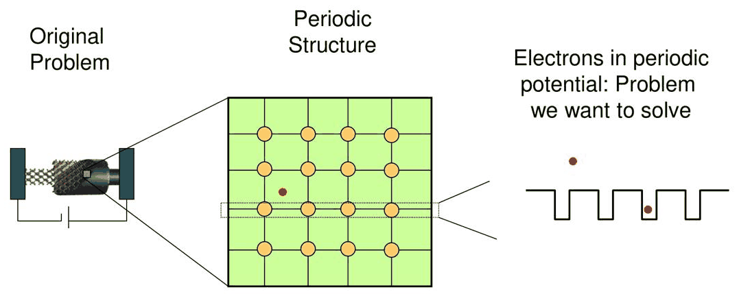
Slide 4: from the device to the periodic potential — Slide 4: a nanowire device, its periodic crystal structure, and the problem to solve: electrons in a periodic potential of square wells.

If the electrons were large objects, like a skier passing a row of obstacles, Newton's mechanics would do. In the micro-world, some electrons sit deep in the buckets, closely bound to the cores; some are loosely bound; and some move above the buckets, freely through the structure. Electrons are waves (Lecture 4.2), and which of them move, and how fast, is a quantum-mechanical question.

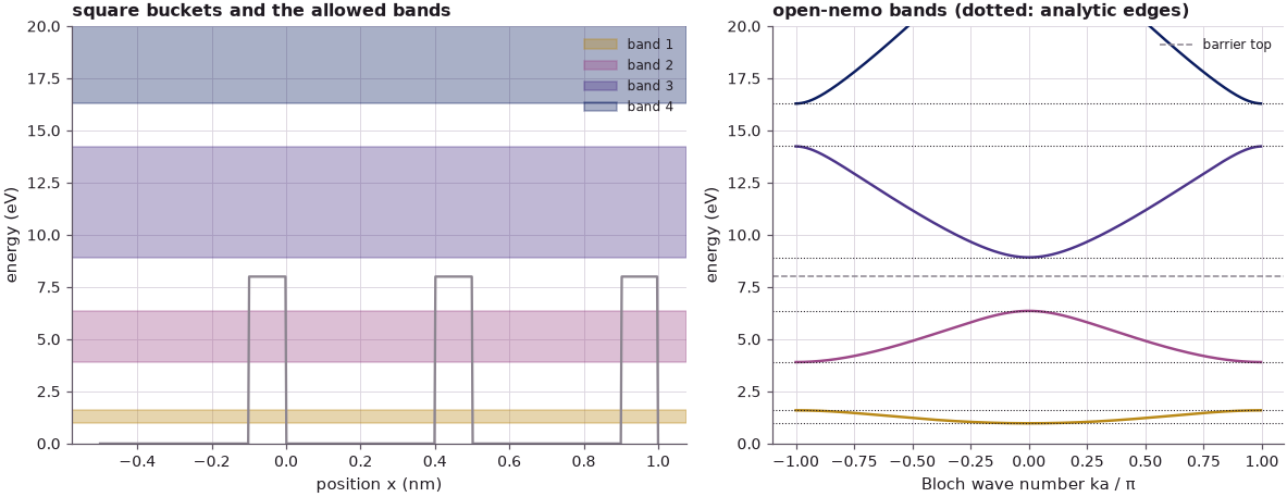
The cell sets up that picture as the Kronig–Penney model: wells of width \(w = 0.4\) nm separated by barriers of height \(U_0 = 8\) eV and width \(b = 0.1\) nm (period \(a = 0.5\) nm, free-electron mass). open-nemo discretizes one period as an effective-mass device, couples it to its periodic copies as a lead, and diagonalizes \(H(q) = h + V e^{iq} + V^\dagger e^{-iq}\) for Bloch phases \(q = ka\). The analytic check is the Kronig–Penney condition (derived in Lecture 7.2):

\cos ka = \cos\alpha w\,\cosh\beta b + \frac{\beta^2 - \alpha^2}{2\alpha\beta}\,\sin\alpha w\,\sinh\beta b, \qquad \alpha = \sqrt{\frac{E}{\hbar^2/2m_0}}, \quad \beta = \sqrt{\frac{U_0 - E}{\hbar^2/2m_0}};

the band edges are the energies where the right side equals ±1 (for \(E > U_0\), \(\beta\) is imaginary and the formula continues analytically).

Code43 lines · cell 3

EM = nemo.structures.materials.EffectiveMassMaterial
w, b, U0, dx = 0.4, 0.1, 8.0, 0.005  # nm, nm, eV, nm
a = w + b
cell = nemo.Heterostructure1D(
    [nemo.Layer(EM("well", 1.0, 1.0), w), nemo.Layer(EM("barrier", 1.0, 1.0, conduction_band_edge=U0), b)],
    spacing=dx,
)
h = cell.hamiltonian.sparse.dense().real
V = np.zeros_like(h)
V[-1, 0] = -HBAR2_2M0 / dx**2  # hopping from the last site of one period to the first site of the next
lead = nemo.Lead(h, V)
q = np.linspace(-np.pi, np.pi, 400, endpoint=False)
bands = np.array([lead.bands(np.array([x]))[0][:4] for x in q])  # (nq, 4) in eV


def kp_rhs(E):
    al, be = np.sqrt(E / HBAR2_2M0 + 0j), np.sqrt((U0 - E) / HBAR2_2M0 + 0j)
    return (
        np.cos(al * w) * np.cosh(be * b) + (be**2 - al**2) / (2 * al * be) * np.sin(al * w) * np.sinh(be * b)
    ).real


Eg = np.linspace(0.01, 45, 90000)
edges = []
for s in (1, -1):
    g = kp_rhs(Eg) - s
    edges += [
        brentq(lambda e: kp_rhs(e) - s, Eg[i], Eg[i + 1])
        for i in np.flatnonzero(np.sign(g[:-1]) != np.sign(g[1:]))
    ]
edges = np.sort(edges)

dq = q[1] - q[0]
v = (np.roll(bands, -1, axis=0) - np.roll(bands, 1, axis=0)) / (2 * dq) * a / HBAR * 1e-9  # (1/ħ) dE/dk, m/s
print(" band   bottom (eV)  analytic   top (eV)  analytic   width (eV)   max |v| (10⁵ m/s)")
for j in range(4):
    lo, hi = bands[:, j].min(), bands[:, j].max()
    print(
        f"{j + 1:4d}   {lo:10.3f}  {edges[2 * j]:8.3f}   {hi:8.3f}  {edges[2 * j + 1]:8.3f}   "
        f"{hi - lo:9.3f}   "
        f"{np.abs(v[:, j]).max() / 1e5:10.1f}"
    )
print(f"free electron at 4 eV for comparison: v = {np.sqrt(2 * 4 * Q / M0) / 1e5:.1f} × 10⁵ m/s")

 band   bottom (eV)  analytic   top (eV)  analytic   width (eV)   max |v| (10⁵ m/s)
   1        0.970     0.971      1.593     1.594       0.623          2.4
   2        3.904     3.905      6.356     6.359       2.453          8.8
   3        8.921     8.924     14.240    14.252       5.319         17.4
   4       16.291    16.300     25.168    25.202       8.878         26.4
free electron at 4 eV for comparison: v = 11.9 × 10⁵ m/s

open-nemo's band edges agree with the Kronig–Penney condition to within 0.012 eV for bands 1–3 and 0.034 eV (0.14 %) at the top of band 4, the discretization error of the 0.005 nm grid, which grows with the energy. The four bands tell Klimeck's story:

Band 1 (0.970–1.593 eV) lies deep in the wells. It is 0.623 eV wide, and its electrons move at most at \(2.4\times10^5\) m/s: they are closely bound to the cores and hop between them only by tunnelling through the barriers.
Band 2 (3.904–6.356 eV) is still below the barrier top but four times wider, with velocities up to \(8.8\times10^5\) m/s: loosely bound.
Bands 3 and 4 (above 8.92 eV) lie above the barriers, where the electrons move freely through the structure. They are wide (5.3 and 8.9 eV), their electrons are faster than a free electron of 4 eV (\(11.9\times10^5\) m/s), and the gaps between them are the only reminder of the lattice.

A classical particle with the energy of band 1 would be trapped in one bucket forever; the quantum electron moves through the whole crystal, only slowly. A classical particle above the barriers would never be reflected; the quantum electron is, at the energies of the gaps.

Code22 lines · cell 5

fig, (a1, a2) = plt.subplots(1, 2, figsize=(11, 4.4), gridspec_kw={"width_ratios": [1.2, 1]})
xs = np.linspace(-a, 2 * a, 600)
a1.plot(xs, np.where(np.mod(xs, a) < w, 0.0, U0), color=style.CONTEXT, lw=1.5)
for j, col in zip(range(4), style.sweep(4)):
    a1.axhspan(bands[:, j].min(), bands[:, j].max(), color=col, alpha=0.35, label=f"band {j + 1}")
a1.set(
    xlabel="position x (nm)", ylabel="energy (eV)", ylim=(0, 20), title="square buckets and the allowed bands"
)
a1.legend(frameon=False, fontsize=8, loc="upper right")
for j, col in zip(range(4), style.sweep(4)):
    a2.plot(q / np.pi, bands[:, j], color=col)
for e in edges[:8]:
    a2.axhline(e, color=style.REFERENCE, ls=":", lw=0.7)
a2.axhline(U0, color=style.CONTEXT, ls="--", lw=1, label="barrier top")
a2.set(
    xlabel="Bloch wave number ka / π",
    ylabel="energy (eV)",
    ylim=(0, 20),
    title="open-nemo bands (dotted: analytic edges)",
)
a2.legend(frameon=False, fontsize=8, loc="upper right")
fig.tight_layout();

Figure computed by the notebook with open-nemo

2. Carrier number = number of states × filling factor#

Knowing the states is half of the answer. Even a free electron can only move if there is an empty state to move into: an electric field shifts electrons from states with \(-k\) to states with \(+k\), and in a completely filled band every state is taken, so the band carries no current, whatever the velocities of its electrons. The number of carriers is therefore

\text{carrier number} = \text{number of states} \times \text{filling factor},

Klimeck's apartment building: the total number of occupants is the number of apartments times the fraction occupied, and the lower floors are full while the upper floors are nearly empty.

Slide 5: carrier number as states times filling — Slide 5: carrier number = number of states × filling factor; the occupants of an apartment building fill the lower floors first.

In equilibrium the filling factor is the Fermi–Dirac function \(f(E) = 1/(1 + e^{(E-E_F)/k_BT})\), with the Fermi level \(E_F\) fixed by the number of electrons. Each band of the crystal holds two electrons per period (one state per period for each spin). The cell fills the Kronig–Penney crystal with 1 to 4 electrons per period at 300 K and measures how many respond to a field. In the relaxation-time picture the conductivity is proportional to

\frac{n_\text{eff}}{m_0} = \frac{2}{L}\sum_{n,k} v_n(k)^2 \left(-\frac{\partial f}{\partial E}\right),

which equals \(n/m_0\) for free electrons of density \(n\). \(n_\text{eff}\), per period, counts the electrons that move like free electrons; only states near \(E_F\) contribute.

Code39 lines · cell 7

kT = KB * 300.0
E_all = bands.ravel()


def electrons_per_period(ef, kt=kT):
    return 2 * np.mean(np.sum(expit((ef - bands) / kt), axis=1))


def n_eff(ef, kt=kT):
    x = (bands - ef) / kt
    minus_df = np.exp(-np.abs(x)) / (1 + np.exp(-np.abs(x))) ** 2 / (kt * Q)  # -df/dE in 1/J, overflow-safe
    return 2 * np.mean(np.sum(M0 * v**2 * minus_df, axis=1))  # per period (dimensionless)


print(" electrons/period   E_F (eV)   band filling                  n_eff per period")
rows = []
for ne in (1, 2, 3, 4):
    ef = brentq(lambda e: electrons_per_period(e) - ne, 0.0, 25.0)
    fill = [2 * np.mean(expit((ef - bands[:, j]) / kT)) for j in range(3)]
    rows.append((ne, ef, n_eff(ef)))
    print(
        f"{ne:10d}         {ef:8.3f}   " + "  ".join(f"{x:5.3f}" for x in fill) + f"         {n_eff(ef):.3e}"
    )

ef_grid = np.linspace(0.5, 10, 400)
fig, (a1, a2) = plt.subplots(1, 2, figsize=(11, 3.8))
a1.plot(ef_grid, [electrons_per_period(e) for e in ef_grid], color=style.OPEN_NEMO)
a1.set(xlabel="Fermi level E_F (eV)", ylabel="electrons per period", title="all electrons: states × filling")
a2.semilogy(ef_grid, [max(n_eff(e), 1e-30) for e in ef_grid], color=style.OPEN_NEMO)
for ne, ef, _ in rows:
    a2.axvline(ef, color=style.sweep(4)[ne - 1], ls=":", label=f"{ne} electron{'s' if ne > 1 else ''}/period")
a2.set(
    xlabel="Fermi level E_F (eV)",
    ylabel="n_eff per period",
    ylim=(1e-30, 10),
    title="electrons that respond to a field",
)
a2.legend(frameon=False, fontsize=8)
fig.tight_layout();

 electrons/period   E_F (eV)   band filling                  n_eff per period
         1            1.226   1.000  0.000  0.000         6.102e-01
         2            2.843   2.000  0.000  0.000         6.468e-19
         3            4.917   2.000  1.000  0.000         2.264e+00
         4            7.471   2.000  2.000  0.000         1.150e-19

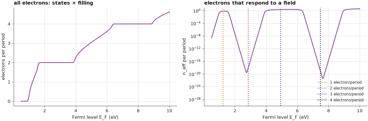
The count of electrons rises in steps of two per band, but the number that responds to a field does not follow it. With 1 or 3 electrons per period a band is half filled, \(E_F\) sits inside it, and the crystal is a metal: \(n_\text{eff}\) is 0.61 and 2.26 electrons per period (smaller than the electron count of the half-filled band 1, whose electrons are heavy and slow; larger than that of band 2, whose curvature is strong). With 2 or 4 electrons per period the bands are exactly full, \(E_F\) lies in a gap, and \(n_\text{eff}\) collapses to \(6.5\times10^{-19}\) and \(1.2\times10^{-19}\): only the electrons thermally lifted across the 2.31 and 2.57 eV gaps can move. The crystal holds the same kind of electrons in all four cases; what differs is whether empty states are available next to them. This is the answer to \(n \ne N\times\rho\), and the reason a semiconductor is described by its bands (the number of states, Chapters 2–3 of the course textbook) and by their filling (statistics, Chapter 4).

3. Outlook: the Schrödinger equation#

Composition and arrangement of the atoms fix the potential; quantum mechanics turns the potential into states and statistical mechanics fills them, which gives the electron density. The next step of the course is the equation that does the first part. Klimeck motivates it rather than deriving it: it arises from the quantization of energy, \(E = hf = \hbar\omega\), and momentum, \(p = \hbar k\), applied to a wave \(e^{i(kx - \omega t)}\) together with the energy relation of a particle. Lecture 5 writes it down and solves the simplest problems: the free electron, the potential step and the particle in a box.

Summary#

An electron in a crystal moves in a periodic potential. In a Kronig–Penney crystal of 8 eV deep, 0.4 nm wide wells, open-nemo's bands agree with the analytic band edges to 0.034 eV or better.
Deep bands are narrow and slow (band 1: 0.623 eV wide, at most \(2.4\times10^5\) m/s), higher bands are wider, and above the barriers the electrons move nearly freely: bound, loosely bound and free electrons in one picture.
Carrier number = number of states × filling. Each band holds 2 electrons per period. With 1 or 3 electrons per period the crystal conducts (\(n_\text{eff}\) = 0.61 and 2.26 per period at 300 K); with 2 or 4 the bands are full and \(n_\text{eff}\) falls below \(10^{-18}\).

Exercises#

Make the barriers thicker (\(b\) = 0.2 nm). How do the width of band 1 and its maximum velocity change? Relate the change to the tunnelling factor \(e^{-\beta b}\).
Raise the temperature to 3000 K in section 2. How large does \(n_\text{eff}\) become for 2 electrons per period, and how does it compare with \(e^{-E_g/2k_BT}\)?
Compare the curvature of band 1 at \(k = 0\) with \(\hbar^2/2m^*\) and find the effective mass \(m^*\). Does \(n_\text{eff}\) for 1 electron per period scale like \(m_0/m^*\)?