

Lecture 1.3
Band structure in nanoelectronics — a basic view
In the lecture
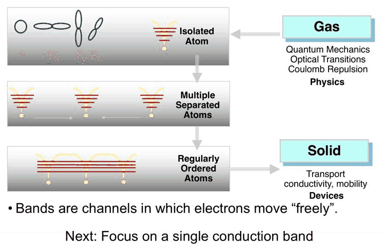
- from atoms to solids: discrete atomic levels broaden into bands, "channels in which electrons move freely"
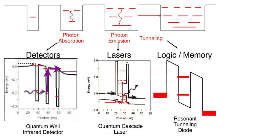
- layers of different materials make barriers and wells; designed band edges give detectors (QWIPs), lasers (quantum cascade lasers) and logic and memory devices (resonant tunneling diodes)
- the materials: GaAs/AlGaAs, InGaAs/InAlAs on InP, and the 6.1 Å family InAs/GaSb/AlSb with its broken gap; Kroemer's "the interface is the device"
- typical device dimensions: an RTD with 4-monolayer AlAs barriers and a 14-monolayer InGaAs well, a few dozen atoms in all
- the band edge diagram, and why quantitative modeling at the nanoscale needs realistic basis states: non-parabolic bands, states at X and L, coupled bands, band wrapping and complex wave vectors
In this notebook
we compute each picture. Coupled quantum wells in open-nemo show discrete levels turning into a band, checked against the Kronig–Penney formula. open-nemo's material registry draws the band gap against lattice constant chart and the band alignments of the three material systems. An effective-mass RTD with the slide's monolayer counts shows how sensitive the resonance is to a single monolayer. Finally sp3d5s* tight binding gives the full, complex band structure of GaAs, compared with the parabolic band and the two-band formula.
Run it on your own machine
The notebook needs open-nemo (Python ≥ 3.10 and a C++20 compiler; BLAS/LAPACK).
git clone https://github.com/denphi/open-nemo.git && cd open-nemo
python3 -m venv .venv && source .venv/bin/activate
pip install -e ".[notebooks]"
jupyter lab From_Atoms_to_Devices/01_introduction/01_3_bandstructure_basic_view.ipynbCode
import numpy as np
import matplotlib.pyplot as plt
import opennemo as nemo
from opennemo.visualization import style

style.use(notebook=True)
from scipy.linalg import eigh_tridiagonal
from opennemo.models import kp
from opennemo.solvers.transport import complex_bands
from opennemo.structures.materials import EffectiveMassMaterial

H2M0 = nemo.core.units.HBAR2_2M0   # ħ²/2m₀ (eV nm²)
props = nemo.structures.properties
1. From atoms to bands#
An isolated atom has discrete levels (s, p, …). Bring several atoms close and their orbitals overlap: each level splits into as many levels as there are atoms. In a regular crystal the levels merge into bands, and an electron in a band is not bound to an atom: bands are the channels in which electrons move "freely". That is the starting point for transport, conductivity and mobility, and thus for devices.
The same physics can be seen with artificial atoms: quantum wells. Here each "atom" is a 5 nm GaAs well between 2 nm barriers 0.324 eV high (the conduction-band offset of Al${0.4}$Ga${0.6}$As in open-nemo's effective-mass set); the mass is 0.067 \(m_0\) everywhere, so that the infinite superlattice has the Kronig–Penney solution
with well width \(a\), barrier width \(b\) and period \(d = a + b\). Energies where the right side lies between −1 and 1 form the allowed bands (minibands). The cell below puts \(N\) wells in a closed box and finds all its levels below the barrier top.
Code
M, A, B = 0.067, 5.0, 2.0                        # mass (m0), well and barrier width (nm)
V0 = nemo.structures.materials.effective_mass("AlGaAs", x=0.4).conduction_band_edge
well = EffectiveMassMaterial("GaAs", M, 12.9)
barrier = EffectiveMassMaterial("Al0.4Ga0.6As (GaAs mass)", M, 12.9, conduction_band_edge=V0)


def box_levels(n):
    # all levels below V0 of n wells in a closed box (n + 1 barriers, hard walls outside them)
    layers = [nemo.Layer(barrier, B)] + [nemo.Layer(well, A), nemo.Layer(barrier, B)] * n
    h = nemo.Heterostructure1D(layers, spacing=0.05).hamiltonian.sparse.matrices[0]
    return eigh_tridiagonal(h.diagonal().real, h.diagonal(1).real, eigvals_only=True,
                            select="v", select_range=(0.0, V0))


def kronig_penney(e):
    q, kap = np.sqrt(M * e / H2M0), np.sqrt(M * (V0 - e) / H2M0)
    return (np.cos(q * A) * np.cosh(kap * B)
            + (kap**2 - q**2) / (2 * q * kap) * np.sin(q * A) * np.sinh(kap * B))


e = np.linspace(1e-4, V0 - 1e-4, 20001)
allowed = np.abs(kronig_penney(e)) <= 1.0
edges = list(e[np.flatnonzero(np.diff(allowed.astype(int)))])
if allowed[-1]:
    edges.append(V0)                             # a band that continues above the barrier top
bands = list(zip(edges[0::2], edges[1::2]))
for i, (lo, hi) in enumerate(bands, 1):
    print(f"Kronig–Penney miniband {i}: {1e3 * lo:6.1f} – {1e3 * hi:6.1f} meV "
          f"(width {1e3 * (hi - lo):5.1f} meV)")

counts = (1, 2, 3, 5, 10, 20)
fig, ax = plt.subplots(figsize=(7, 4))
for lo, hi in bands:
    ax.axhspan(1e3 * lo, 1e3 * hi, color=style.REFERENCE, alpha=0.15, lw=0)
for j, n in enumerate(counts):
    lv = box_levels(n)
    ax.hlines(1e3 * lv, j - 0.3, j + 0.3, color=style.OPEN_NEMO, lw=1)
    inside = [int(np.sum((lv >= lo - 1e-3) & (lv <= hi + 1e-3))) for lo, hi in bands]
    print(f"N = {n:2d} wells: {len(lv):2d} levels below V0; per miniband {inside}; "
          f"lowest {1e3 * lv[0]:.1f} meV")
ax.set_xticks(range(len(counts)), [str(n) for n in counts])
ax.set(xlabel="number of wells N", ylabel="energy (meV)", ylim=(0, 1e3 * V0))
ax.set_title("levels of N coupled wells (lines) and Kronig–Penney minibands (shaded)", fontsize=10)
fig.tight_layout()
Kronig–Penney miniband 1:   66.7 –  125.1 meV (width  58.3 meV)
Kronig–Penney miniband 2:  266.8 –  324.2 meV (width  57.4 meV)
N =  1 wells:  1 levels below V0; per miniband [1, 0]; lowest 100.5 meV
N =  2 wells:  3 levels below V0; per miniband [2, 1]; lowest 81.1 meV
N =  3 wells:  4 levels below V0; per miniband [3, 1]; lowest 74.3 meV
N =  5 wells:  7 levels below V0; per miniband [5, 2]; lowest 69.8 meV
N = 10 wells: 14 levels below V0; per miniband [10, 4]; lowest 67.6 meV
N = 20 wells: 27 levels below V0; per miniband [20, 7]; lowest 66.9 meV
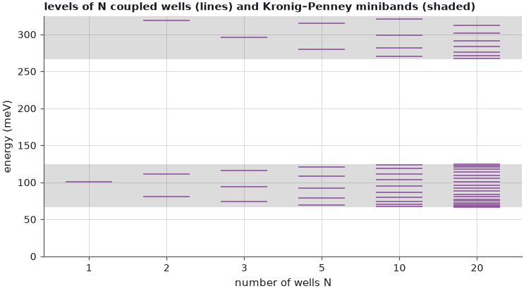
One well has a single bound level, at 100.5 meV. With \(N\) wells it splits into \(N\) levels, all inside the lower miniband of the infinite superlattice (shaded, 66.7–125.1 meV, 58 meV wide); as \(N\) grows they fill it, and the lowest approaches its bottom (66.9 meV for 20 wells). The width measures how strongly neighbouring wells (atoms) couple, and the levels never leave the band, no matter how many wells are added. More levels appear from 267 meV: the second miniband, which in the coupled system starts below the barrier top although a single well has no second bound state. Real atoms couple more strongly and have several orbitals, which is why real bands are electron-volts wide — and why the full band structure is needed later.
2. Transitions and transport controlled by design#
Once the band edge can be shaped layer by layer, its levels can be placed where a device needs them. An electron in a well can absorb a photon and leave (a quantum well infrared photodetector, QWIP), drop between designed levels and emit one (a quantum cascade laser, QCL), or tunnel through a double barrier when a level lines up with the emitter (a resonant tunneling diode, RTD, the example of the course). The Nobel prize in physics 2000 went half to Jack Kilby for the integrated circuit and a quarter each to Zhores Alferov and Herbert Kroemer for semiconductor heterostructures; Kroemer's phrase for it is "the interface is the device".
3. Materials: band gaps, lattice constants and alignments#
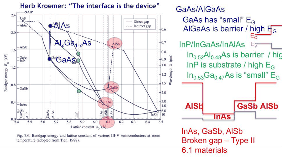
The layers must grow on each other without defects, which in practice means nearly the same lattice constant. Slide 12 shows the classic chart of band gap against lattice constant. The cell below draws it again from open-nemo's property registry (300 K values; Γ gaps of the binaries, alloys joined by the registry's interpolation with bowing).
Code
binaries = ["GaP", "AlP", "GaAs", "AlAs", "InP", "InAs", "GaSb", "AlSb", "InSb"]
alloys = ["AlGaAs", "InGaAs", "InAlAs", "GaInP", "AlInP", "GaAsP", "InAsP", "GaAsSb", "InAsSb",
          "AlAsSb", "AlGaSb", "GaInSb"]
xs = np.linspace(0.0, 1.0, 51)
fig, ax = plt.subplots(figsize=(7.5, 5))
for name in alloys:
    a = [props.value(name, "lattice_constant", x=x) for x in xs]
    g = [props.value(name, "band_gap", x=x) for x in xs]
    ax.plot(10 * np.array(a), g, color=style.CONTEXT, lw=0.8)
for name in binaries:
    a, g = 10 * props.value(name, "lattice_constant"), props.value(name, "band_gap")
    ax.plot(a, g, "o", color=style.OPEN_NEMO, ms=5)
    ax.annotate(name, (a, g), textcoords="offset points", xytext=(4, 4), fontsize=8)
a_inp = 10 * props.value("InP", "lattice_constant")
ax.axvline(a_inp, color=style.REFERENCE, ls="--", lw=0.8)
ax.axvspan(6.05, 6.15, color=style.REFERENCE, alpha=0.1, lw=0)
for name, x in (("AlGaAs", 0.4), ("InGaAs", 0.53), ("InAlAs", 0.52)):
    a, g = 10 * props.value(name, "lattice_constant", x=x), props.value(name, "band_gap", x=x)
    ax.plot(a, g, "s", color=style.sweep(3)[1], ms=5)
    print(f"{name} (x = {x}): a = {a:.4f} Å, E_g = {g:.3f} eV")
ax.set(xlabel="lattice constant a (Å)", ylabel="direct (Γ) band gap $E_g$ (eV)", ylim=(0, 3.7))
fig.tight_layout()
print(f"InP: a = {a_inp:.4f} Å;  GaAs/AlAs mismatch "
      f"{100 * (props.value('AlAs', 'lattice_constant') / props.value('GaAs', 'lattice_constant') - 1):.2f}"
      " %")
AlGaAs (x = 0.4): a = 5.6564 Å, E_g = 1.959 eV
InGaAs (x = 0.53): a = 5.8679 Å, E_g = 0.737 eV
InAlAs (x = 0.52): a = 5.8676 Å, E_g = 1.451 eV
InP: a = 5.8697 Å;  GaAs/AlAs mismatch 0.14 %
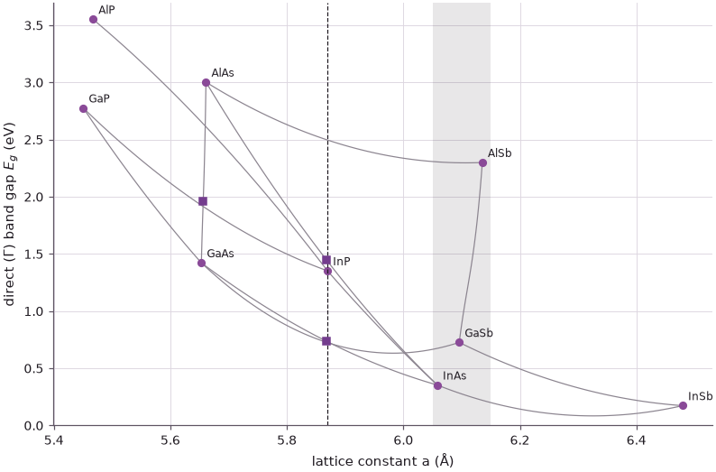
GaAs and AlAs have nearly the same lattice constant (0.14 % apart), so Al$x$Ga${1-x}$As grows on GaAs at any composition: the GaAs/AlGaAs system of slide 12, with GaAs as the small-gap well and AlGaAs as the barrier. In${0.53}$Ga${0.47}$As (small gap) and In${0.52}$Al${0.48}$As (barrier) both match InP (dashed line), the substrate. The shaded strip at 6.1 Å holds InAs, GaSb and AlSb. (The chart shows the direct gaps; AlAs, AlSb and GaP are indirect, and their lowest conduction band is at X or L, below the Γ value plotted.)
What matters for a device is not the gap alone but how the band edges line up. The registry gives each material's valence-band edge on a common scale (the valence band offset); the conduction band edge is that plus the gap.
Code
systems = {
    "GaAs / AlGaAs": [("Al0.4Ga0.6As", "AlGaAs", 0.4), ("GaAs", "GaAs", None),
                      ("Al0.4Ga0.6As", "AlGaAs", 0.4)],
    "InGaAs / InAlAs on InP": [("InP", "InP", None), ("In0.52Al0.48As", "InAlAs", 0.52),
                               ("In0.53Ga0.47As", "InGaAs", 0.53), ("In0.52Al0.48As", "InAlAs", 0.52)],
    "6.1 Å: InAs / GaSb / AlSb": [("AlSb", "AlSb", None), ("InAs", "InAs", None),
                                  ("GaSb", "GaSb", None), ("AlSb", "AlSb", None)],
}


def edges(name, x):
    kw = {} if x is None else {"x": x}
    ev = props.value(name, "valence_band_offset", **kw)
    return ev + props.value(name, "band_gap", **kw), ev


fig, axes = plt.subplots(1, 3, figsize=(12, 3.8), sharey=True)
for ax, (title, layers) in zip(axes, systems.items()):
    for j, (label, name, x) in enumerate(layers):
        ec, ev = edges(name, x)
        ax.hlines(ec, j, j + 1, color=style.OPEN_NEMO, lw=2)
        ax.hlines(ev, j, j + 1, color=style.REFERENCE, lw=2)
        ax.text(j + 0.5, ec + 0.05, label, ha="center", fontsize=7)
    ax.set_title(title, fontsize=10)
    ax.set_xticks([])
axes[0].set(ylabel="band edge (eV, common valence-band scale)")
axes[0].plot([], [], color=style.OPEN_NEMO, lw=2, label="conduction band $E_c$ (Γ)")
axes[0].plot([], [], color=style.REFERENCE, lw=2, label="valence band $E_v$")
axes[0].legend(fontsize=8, loc="center left")
fig.tight_layout()

for a, b in (("GaAs", None), ("AlGaAs", 0.4)), (("InGaAs", 0.53), ("InAlAs", 0.52)):
    (ec1, ev1), (ec2, ev2) = edges(*a), edges(*b)
    print(f"{a[0]}/{b[0]}: ΔE_c = {ec2 - ec1:.3f} eV, ΔE_v = {ev1 - ev2:.3f} eV, "
          f"ΔE_c/ΔE_g = {(ec2 - ec1) / (ec2 - ev2 - ec1 + ev1):.2f}")
ec_inas, ev_gasb = edges("InAs", None)[0], edges("GaSb", None)[1]
print(f"InAs conduction edge {ec_inas:.3f} eV lies {ev_gasb - ec_inas:.3f} eV below the GaSb valence edge "
      f"{ev_gasb:.3f} eV: a broken (type II) gap")
GaAs/AlGaAs: ΔE_c = 0.325 eV, ΔE_v = 0.212 eV, ΔE_c/ΔE_g = 0.61
InGaAs/InAlAs: ΔE_c = 0.522 eV, ΔE_v = 0.191 eV, ΔE_c/ΔE_g = 0.73
InAs conduction edge -0.236 eV lies 0.206 eV below the GaSb valence edge -0.030 eV: a broken (type II) gap
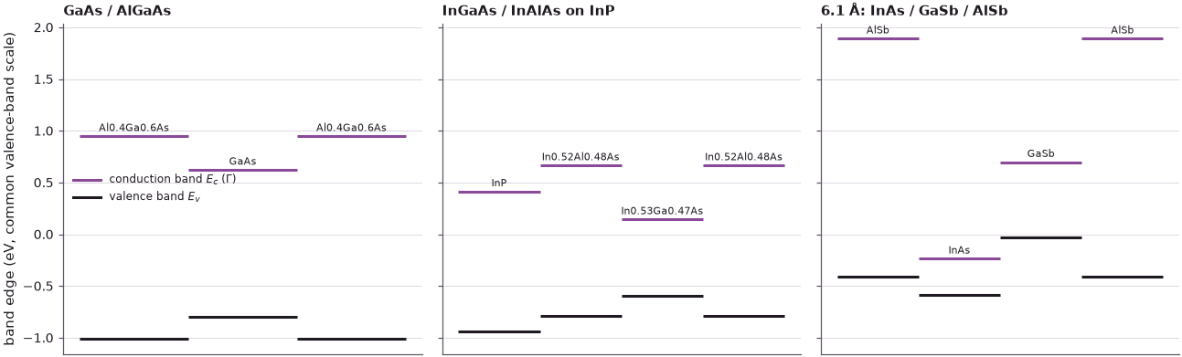
GaAs/Al${0.4}$Ga${0.6}$As and In${0.53}$Ga${0.47}$As/In${0.52}$Al${0.48}$As are type I alignments: the small-gap material is a well for both electrons and holes. The InGaAs/InAlAs pair has the larger conduction-band offset, about 0.52 eV against 0.33 eV, which is one reason it is preferred for RTDs and high-speed transistors. InAs/GaSb is different in kind: the InAs conduction band lies about 0.2 eV below the GaSb valence band, so electrons in InAs and holes in GaSb sit next to each other at the same energy — the broken gap. An electron can pass from a conduction band into a valence band, a coupling that no single-band model contains.
Klimeck contrasts two statements: "if you cannot draw a band edge diagram, you don't understand your device" (a common saying, and true), and his own, "quantitative modeling at the nanoscale requires realistic basis states". The rest of the notebook shows why the second follows.
4. Typical device dimensions: monolayers and atoms#
Slide 15 gives the dimensions of an InGaAs/AlAs RTD grown on InP: two AlAs barriers 1.2 nm thick, 4 monolayers (ML) or 8 atoms along the growth direction, around an In${0.53}$Ga${0.47}$As well 4.2 nm thick, 14 ML or 28 atoms. A monolayer is one cation–anion pair, \(a/2\) thick in the [001] direction.
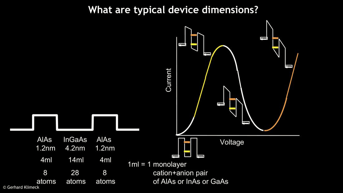
Layer thicknesses are integer numbers of monolayers: a device can only be one monolayer thicker or thinner. How much does that matter? The cell builds the RTD in the effective-mass approximation (Γ-valley masses and offsets from open-nemo's k·p parameters, the AlAs barriers taken unstrained) and computes the lowest resonance of the double barrier for wells of 12 to 16 ML.
Code
ml = props.value("InP", "lattice_constant") / 2           # one monolayer on InP (nm)
ingaas, alas = kp.material("InGaAs", x=0.53), kp.material("AlAs")
ec_w = ingaas.valence_band_offset + ingaas.band_gap
ec_b = alas.valence_band_offset + alas.band_gap               # Γ conduction edge of AlAs
w_mat = EffectiveMassMaterial("In0.53Ga0.47As", ingaas.electron_mass, ingaas.eps_r)
b_mat = EffectiveMassMaterial("AlAs (Γ)", alas.electron_mass, alas.eps_r, conduction_band_edge=ec_b - ec_w)
print(f"1 ML = {ml:.4f} nm;  4 ML = {4 * ml:.2f} nm, 14 ML = {14 * ml:.2f} nm")
print(f"m*(InGaAs) = {ingaas.electron_mass:.4f}, m*(AlAs, Γ) = {alas.electron_mass:.3f} m0, "
      f"ΔE_c(Γ) = {ec_b - ec_w:.3f} eV")


def rtd(n_well, n_bar=4, lead=40):
    lay = [nemo.Layer(w_mat, lead * ml), nemo.Layer(b_mat, n_bar * ml), nemo.Layer(w_mat, n_well * ml),
           nemo.Layer(b_mat, n_bar * ml), nemo.Layer(w_mat, lead * ml)]
    return nemo.Heterostructure1D(lay, spacing=ml / 4)


print("\nwell (ML)  well (nm)  E_1 (meV)  width Γ_1 (meV)  infinite well (meV)")
first = {}
for n in (12, 13, 14, 15, 16):
    res = nemo.resonances(rtd(n))
    k = np.argmin(np.abs(res["energy"] - 0.0) + 1e9 * (res["energy"] <= 0))
    first[n] = res["energy"][k]
    inf = H2M0 * np.pi**2 / (ingaas.electron_mass * (n * ml) ** 2)
    print(f"{n:6d}  {n * ml:9.2f}  {1e3 * first[n]:9.1f}  {1e3 * res['width'][k]:14.3f}  {1e3 * inf:15.0f}")
print(f"one monolayer more or less around 14 ML: {1e3 * (first[13] - first[14]):+.1f} / "
      f"{1e3 * (first[15] - first[14]):+.1f} meV")
1 ML = 0.2935 nm;  4 ML = 1.17 nm, 14 ML = 4.11 nm
m*(InGaAs) = 0.0430, m*(AlAs, Γ) = 0.150 m0, ΔE_c(Γ) = 1.530 eV

well (ML)  well (nm)  E_1 (meV)  width Γ_1 (meV)  infinite well (meV)
    12       3.52      231.5           2.968              705
    13       3.82      209.6           2.483              601
    14       4.11      190.8           2.096              518
    15       4.40      174.5           1.783              451
    16       4.70      160.3           1.526              397
one monolayer more or less around 14 ML: +18.8 / -16.3 meV
One monolayer more or less in a 14 ML well moves the resonance by 16–19 meV, about \(0.7\,k_BT\) at room temperature, and the peak of the current–voltage curve moves with it by roughly twice that in bias. A device is defined to the atom. And the effective-mass numbers themselves are suspect: the resonance sits 0.19 eV above the InGaAs band edge, where its band is no longer parabolic (the infinite-well estimate in the last column is far off for the opposite reason: the wave function leaks into the barriers), and inside 4 ML of AlAs the electron's decaying wave function is set by the band structure in the gap — the complex bands of the next section. Lecture 2 tells the story of RTDs whose modeling, done with full band structure, was more accurate than the growth.
5. Full band structure against parabolic bands#
The standard description of a semiconductor is the band edge \(E_c\) and an effective mass \(m^*\): \(E = E_c + \hbar^2k^2/2m^*\), decoupled parabolic bands. It is the basis of drift–diffusion, Boltzmann transport and most quantum transport simulators. It fails where the nanoscale probes the band away from its minimum: the conduction band is non-parabolic, there are states at X and L, the valence band is not simple, and the bands are coupled. Solving \(H\Psi = E\Psi\) with plane-wave solutions \(\Psi \propto e^{ikr}\) gives \(E(k)\) for real \(k\) (propagating states) but also for imaginary \(k = i\kappa\), \(\Psi \propto e^{-\kappa r}\): the evanescent states that carry tunneling through a barrier. In the gap, \(\kappa(E)\) connects the conduction band to the valence band — band wrapping — while the parabolic band's \(\kappa\) grows without limit.
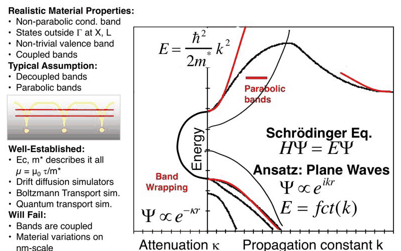
The cell computes the complex band structure of bulk GaAs along [001] with the sp3d5s* tight
binding parameters of nemo5_sp3d5s_so (10 orbitals per atom), and compares it with the
parabolic band (\(m^* = 0.067\,m_0\)) and with the two-band (Franz) formula
\(\kappa^2 = \frac{2m^*}{\hbar^2}\frac{(E_c - E)(E - E_v)}{E_g}\), the simplest model that wraps.
Code
gaas = nemo.structures.materials.load("nemo5_sp3d5s_so")["GaAs"]
lat = nemo.structures.lattice.from_material(gaas)
dev = nemo.Device(lat, cells=(2, 1, 1), periodic=("y", "z"))
lead = nemo.models.tb.SlaterKoster(gaas).partition(dev).lead(k=np.zeros(3))
energies = np.linspace(-0.6, 2.0, 521)
cb = complex_bands(lead, energies, period=gaas.lattice_constant)
kr, ki = np.asarray(cb["k_real"]), np.asarray(cb["k_imag"])
prop = np.abs(ki) < 1e-6                                  # propagating (real k) solutions

# band edges at Γ, and the conduction-band mass from the smallest real k just above E_c
kmin_real = np.where(prop, np.abs(kr), np.inf).min(axis=1)
kmin_real[np.isinf(kmin_real)] = np.nan             # no propagating state: inside the gap
kappa = np.where(~prop & (np.abs(kr) < 1e-6), np.abs(ki), np.inf).min(axis=1)
kappa[np.isinf(kappa)] = np.nan
gap = np.isnan(kmin_real)
ev, ec = energies[~gap & (energies < 0.7)].max(), energies[~gap & (energies > 0.7)].min()
print(f"TB band edges on this grid: E_v = {ev:.3f} eV, E_c = {ec:.3f} eV, E_g = {ec - ev:.3f} eV")
for de in (0.02, 0.1, 0.2, 0.3):
    j = np.argmin(np.abs(energies - (ec + de)))
    k = kmin_real[j]
    print(f"E - E_c = {energies[j] - ec:.3f} eV: k = {k:.3f} 1/nm "
          f"(parabolic {np.sqrt(0.067 * de / H2M0):.3f}), "
          f"mass from E = ħ²k²/2m: {H2M0 * k**2 / (energies[j] - ec):.3f} m0")

eg = ec - ev
e_gap = energies[gap]
k_par = np.sqrt(0.067 * (ec - e_gap) / H2M0)
k_franz = np.sqrt(0.067 * (ec - e_gap) * (e_gap - ev) / (eg * H2M0))
j = np.argmin(np.abs(e_gap - (ev + ec) / 2))
print(f"mid-gap: κ TB = {kappa[gap][j]:.3f}, two-band {k_franz[j]:.3f}, parabolic {k_par[j]:.3f} 1/nm")
print(f"largest κ in the gap (TB): {np.nanmax(kappa[gap]):.3f} 1/nm "
      f"at E = {e_gap[np.nanargmax(kappa[gap])]:.3f} eV")

fig, ax = plt.subplots(figsize=(7.5, 5))
for col in range(kr.shape[1]):
    sel = prop[:, col] & (np.abs(kr[:, col]) < 2.5)
    ax.plot(np.abs(kr[sel, col]), energies[sel], ".", color=style.OPEN_NEMO, ms=1.5)
ax.plot(-kappa, energies, ".", color=style.OPEN_NEMO, ms=1.5, label="sp3d5s* tight binding")
k_up = np.linspace(0, 2.5, 200)
ax.plot(k_up, ec + H2M0 * k_up**2 / 0.067, color=style.REFERENCE, lw=1, label="parabolic, $m^*$ = 0.067")
ax.plot(-k_par, e_gap, color=style.REFERENCE, lw=1)
ax.plot(-k_franz, e_gap, color=style.sweep(3)[1], lw=1, ls="--", label="two-band (Franz) κ")
ax.axvline(0, color=style.CONTEXT, lw=0.8)
ax.set(xlabel="attenuation κ (1/nm, left)   |   propagation constant k (1/nm, right)",
       ylabel="energy (eV)", xlim=(-2.5, 2.5), ylim=(energies[0], energies[-1]))
ax.legend(fontsize=8, loc="lower right", markerscale=6)
fig.tight_layout()
TB band edges on this grid: E_v = -0.110 eV, E_c = 1.425 eV, E_g = 1.535 eV
E - E_c = 0.020 eV: k = 0.193 1/nm (parabolic 0.188), mass from E = ħ²k²/2m: 0.071 m0
E - E_c = 0.100 eV: k = 0.436 1/nm (parabolic 0.419), mass from E = ħ²k²/2m: 0.073 m0
E - E_c = 0.200 eV: k = 0.636 1/nm (parabolic 0.593), mass from E = ħ²k²/2m: 0.077 m0
E - E_c = 0.300 eV: k = 0.803 1/nm (parabolic 0.726), mass from E = ħ²k²/2m: 0.082 m0
mid-gap: κ TB = 0.810, two-band 0.821, parabolic 1.164 1/nm
largest κ in the gap (TB): 0.810 1/nm at E = 0.665 eV
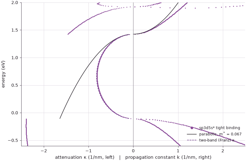
The calculation leaves out spin (the default of SlaterKoster), so the spin–orbit splitting is
missing and the valence-band top sits about a third of it lower than in the real crystal: the
printed gap is 1.535 eV instead of 1.42 eV. That does not change the picture. Near the band edge
the tight-binding conduction band and the parabola agree: the mass from
\(E = \hbar^2k^2/2m\) is 0.071 \(m_0\) at 20 meV. Higher up the band bends away: the same formula
gives 0.077 \(m_0\) at 0.2 eV and 0.082 \(m_0\) at 0.3 eV, about 15 % heavier than at the edge — the
non-parabolicity that the resonance of Section 4 sits in (in InGaAs, with its smaller gap, it is
stronger). In the gap the difference is
qualitative. The tight-binding \(\kappa\) rises from zero at \(E_c\), reaches its maximum near
mid-gap and falls back to zero at the valence band: it wraps. The parabolic \(\kappa\) keeps growing
and at mid-gap overestimates the attenuation by 44 % (1.16 against 0.81 nm⁻¹); the two-band
formula, which builds in the coupling of the conduction and light-hole bands, follows the
tight-binding curve to about 1 % at mid-gap. (The other branches in the figure are evanescent and
propagating states of the remote bands, for example the folded X-valley states near 1.9 eV.)
Tunneling currents depend exponentially on \(\kappa\) times the barrier thickness, so these
differences are orders of magnitude in current.
6. From materials to devices#
Slides 16–22 sketch what comes next in the course. A 15-atom chain in a box previews the particle-in-a-box of Section 9 of the course, the sp3d5s* basis connects materials to devices ("empirical tight binding makes the connection between materials and devices"), and the crystal itself is not symmetric along the growth direction (the cation and anion planes alternate). Klimeck recalls a 1998 challenge from Robert Dutton of Stanford — "talk to me again when you do this in 3D" — which led to NEMO3D and NEMO5, used in industry from 2015.
Summary#
- \(N\) coupled quantum wells give \(N\) levels per bound state of one well, all inside the Kronig–Penney minibands of the infinite superlattice: levels become bands.
- open-nemo's registry reproduces the gap–lattice-constant chart; InGaAs/InAlAs (lattice matched to InP) has a conduction-band offset of 0.52 eV against 0.33 eV for GaAs/Al${0.4}$Ga${0.6}$As, and InAs/GaSb has a broken gap of about 0.2 eV.
- In an InGaAs/AlAs RTD with 4 ML barriers, one monolayer of well width moves the resonance by 16–19 meV, the resonance being 0.19 eV above the band edge.
- The sp3d5s* complex band structure of GaAs shows non-parabolicity (a mass about 15 % heavier at 0.3 eV) and band wrapping in the gap, which the parabolic band misses and the two-band formula captures.
Exercises#
- Make the barriers of Section 1 thinner (1 nm) and thicker (4 nm). How do the miniband widths change? Relate the change to \(e^{-2\kappa b}\).
- Use the Al${0.4}$Ga${0.6}$As mass (0.0919 \(m_0\)) in the barriers and compare the closed-box levels with the equal-mass Kronig–Penney bands. Which boundary condition does open-nemo use?
- Compute the RTD resonances with 3 and 5 ML barriers. Which quantity is more sensitive to one monolayer: the resonance energy or its width?
- Repeat the complex band structure for Si with
boykin2004_sp3d5salong [001]. Where are the real-k conduction states, and how does the evanescent branch in the gap differ from GaAs?
Further reading#
- Bands from coupled wells
- Effective masses and non-parabolicity
- Material property registry
- Atomistic against effective-mass RTD
- Broken-gap heterostructures: k·p against tight binding
- H. Kroemer, "Quasi-electric fields and band offsets: teaching electrons new tricks", Nobel lecture, Rev. Mod. Phys. 73, 783 (2001).
- I. Vurgaftman, J. R. Meyer and L. R. Ram-Mohan, J. Appl. Phys. 89, 5815 (2001) (band parameters).
- P. K. Tien, Integrated Optics and New Wave Phenomena in Optical Waveguides (1988), the source of the chart on slide 12.
- T. B. Boykin, G. Klimeck, R. C. Bowen and F. Oyafuso, "Diagonal parameter shifts due to nearest- neighbor displacements in empirical tight-binding theory", Phys. Rev. B 66, 125207 (2002).