

ECE 606 Lecture 2.1
Typical semiconducting materials
In the lecture
- the goal of the course, the current \(I = G\,V = q\,n\,v\,A\), and why the charge density \(n\) and the velocity \(v\) start with the materials
- why tabulated bulk properties are not enough at the nanometre scale, where composition, strain and geometry change them: quantum mechanics and statistical mechanics are needed
- the two things a material contributes: its atomic composition (electrons per atom) and the arrangement of its atoms (which decides how many electrons can conduct)
- the periodic table: shells fill from left to right, new shells are added from top to bottom; Si and Ge sit in column IV with half-filled s and p shells
- compound semiconductors: III–V and II–VI pairs that share electrons so that each atom has four valence electrons on average
In this notebook
counts atoms, electrons and valence electrons per volume in the open-nemo Si crystal and shows that far fewer electrons carry current than the crystal holds; it then computes the band gaps of the column-IV and III–V semiconductors with sp3d5s* tight binding and arranges them like the periodic table of the lecture: the gap shrinks down a column and grows from IV to III–V to II–VI along a row.
Run it on your own machine
The notebook needs open-nemo (Python ≥ 3.10 and a C++20 compiler; BLAS/LAPACK).
git clone https://github.com/denphi/open-nemo.git && cd open-nemo
python3 -m venv .venv && source .venv/bin/activate
pip install -e ".[notebooks]"
jupyter lab From_Atoms_to_Devices/02_materials_and_quantum_mechanics/02_1_typical_semiconducting_materials.ipynbCode
import numpy as np
import matplotlib.pyplot as plt
import opennemo as nemo
from opennemo.visualization import style

style.use(notebook=True)
1. Current flow needs a charge density and a velocity#
The whole course is after one quantity: the current \(I\) that flows through a device when a voltage \(V\) is applied. Ohm's law writes it as \(I = G\,V\), with the conductance \(G\). Klimeck breaks it into the factors that the physics has to supply:
with the elementary charge \(q = 1.602\times10^{-19}\) C, the density \(n\) of the electrons that move (cm⁻³), their velocity \(v\) (cm/s) and the cross-section \(A\) (cm²) of the conductor. The course follows these factors in order. First the materials: their composition and crystal structure, which for bulk materials are tabulated, but which at the nanometre scale change with geometry, strain and composition, so that they have to be computed with quantum mechanics and equilibrium statistical mechanics (effective masses, occupation factors). Then transport, with scattering and non-equilibrium statistical mechanics (drift–diffusion with recombination and generation). Finally concrete devices: diodes, bipolar transistors and MOSFETs.

2. Atomic composition and arrangement of atoms#
A material brings two things to \(n\): its atomic composition, which fixes the number of electrons per atom, and the arrangement of its atoms, which fixes the number of atoms per volume and, through the bonds, how many of the electrons are free to conduct. Klimeck stresses that not all electrons are available for conduction.
Silicon makes this concrete. Its atoms sit on the diamond lattice (two atoms per primitive cell), each atom has \(Z = 14\) electrons, ten of them in the closed shells \(1s^2 2s^2 2p^6\) and four in the valence shell \(3s^2 3p^2\). The cell below builds the open-nemo Si crystal (lattice constant of the Jancu 1998 tight-binding set) and counts.
Code
JANCU = nemo.structures.materials.load("jancu1998_sp3d5s")  # sp3d5s* (+ spin–orbit): IV and III–V
si = JANCU["Si"]
lat = nemo.structures.lattice.from_material(si)
v_cell = abs(np.linalg.det(lat.vectors))  # primitive-cell volume (nm³)
rho = len(lat.basis) / v_cell * 1e21  # atoms per cm³ (1 nm³ = 1e-21 cm³)
bonds = lat.bond_vectors[0]
cos = bonds @ bonds.T / np.linalg.norm(bonds, axis=1) ** 2
print(f"a = {si.lattice_constant} nm, {len(lat.basis)} atoms per primitive cell of {v_cell:.5f} nm³")
print(f"atoms:              {rho:.3e} cm⁻³  (= 8/a³)")
print(f"all electrons:      {14 * rho:.3e} cm⁻³  (Z = 14)")
print(f"valence electrons:  {4 * rho:.3e} cm⁻³  (3s² 3p²)")
print(
    f"{len(bonds)} nearest neighbours at {lat.nearest_neighbor_distance:.4f} nm, "
    f"bond angle {np.degrees(np.arccos(cos[0, 1])):.2f}°"
)

# if every valence electron moved at the saturation velocity through a 10 nm × 10 nm wire:
q, v_sat, area = 1.602e-19, 1e7, (10e-7) ** 2  # C, cm/s, cm²
print(f"\nI = q n v A with all valence electrons: {q * 4 * rho * v_sat * area:.2f} A")
a = 0.543 nm, 2 atoms per primitive cell of 0.04003 nm³
atoms:              4.997e+22 cm⁻³  (= 8/a³)
all electrons:      6.995e+23 cm⁻³  (Z = 14)
valence electrons:  1.999e+23 cm⁻³  (3s² 3p²)
4 nearest neighbours at 0.2351 nm, bond angle 109.47°

I = q n v A with all valence electrons: 0.32 A
Silicon has \(5.0\times10^{22}\) atoms and \(2.0\times10^{23}\) valence electrons per cm³. If all of them moved at the saturation velocity of \(10^7\) cm/s, a wire of only 10 nm × 10 nm cross-section would carry 0.32 A. Nanowire transistors of that size deliver currents of the order of 10 µA, about \(10^{-4}\) of this. The density of electrons that actually move is set by the bonds, the bands and their filling: that is what the next lectures develop. In Klimeck's words, all electrons may be created equal, but they do not behave identically.
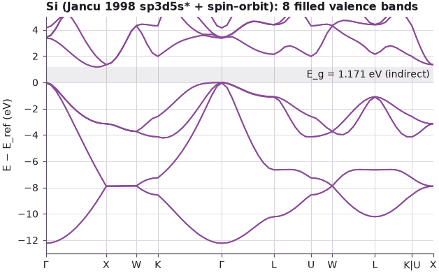
Each Si atom has four nearest neighbours at 0.235 nm, at the tetrahedral angle of 109.47°: one bond for each of its four valence electrons. In the tight-binding model this shows as a count of states. The model keeps only the valence orbitals of each atom; with spin, two atoms give 8 valence bands, which hold exactly the 8 valence electrons of the cell. The 8 bands are full, the gap above them is empty, and a full band carries no net current.
Code
h_si = nemo.models.tb.SlaterKoster(si, spin=True).build(nemo.structures.structure.bulk(lat))
path = nemo.structures.kpath.auto(lat.periods, 80)
g = nemo.band_gap(h_si, path, num_occupied=8)
print(
    f"{h_si.dense(np.zeros(3)).shape[0]} bands (10 orbitals × 2 atoms × 2 spins), 8 occupied; "
    f"gap {g['gap']:.3f} eV, {'direct' if g['direct'] else 'indirect'}"
)
fig, ax = plt.subplots(figsize=(6.5, 4))
nemo.visualization.viz.bands(
    nemo.bands(h_si, path), ax=ax, num_occupied=8, reference="vbm", energy_range=(-13, 5)
)
ax.set_title("Si (Jancu 1998 sp3d5s* + spin–orbit): 8 filled valence bands");
40 bands (10 orbitals × 2 atoms × 2 spins), 8 occupied; gap 1.170 eV, indirect
3. Elemental semiconductors in the periodic table#
Klimeck reads the periodic table along two directions. From left to right the electron shells fill up, and the atoms become heavier. From top to bottom new shells are added, and the atoms become heavier and larger. Column VIII (the noble gases) has full shells: a "happy" configuration in which all electrons are bound. Column IV, with C, Si, Ge and Sn, has its outer s and p shells exactly half filled: 4 of the 8 places of \(s^2p^6\) are occupied. Si and Ge are the elemental semiconductors.
Be and Mg appear at the far left of the full table but, like Zn, Cd and Hg, they are column-II elements filling the same s and p shells. It is convenient to cut the table down to columns II to VI.

Going down column IV the atoms grow, the lattice constant grows, the bonds become weaker, and the gap between the filled and the empty bands shrinks: diamond is an insulator, Si and Ge are semiconductors, and grey (α) tin is a semimetal without a gap. The cell computes this trend with the sp3d5s* + spin–orbit parameters of Jancu et al. (1998), which were fitted to the measured band structures at low temperature.
Code
def tb_gap(mat):
    """Band gap of a zincblende or diamond material (sp3d5s* + spin–orbit, 8 valence bands)."""
    lt = nemo.structures.lattice.from_material(mat)
    h = nemo.models.tb.SlaterKoster(mat, spin=True).build(nemo.structures.structure.bulk(lt))
    r = nemo.band_gap(h, nemo.structures.kpath.auto(lt.periods, 40), num_occupied=8)
    return r["gap"], r["direct"], lt.nearest_neighbor_distance


TB = {name: (m.lattice_constant, *tb_gap(m)) for name, m in JANCU.materials.items()}
print("column IV     a (nm)   d_nn (nm)   gap (eV)")
for name in ("C", "Si", "Ge"):
    a, gap, direct, dnn = TB[name]
    print(f"{name:10s}  {a:8.4f}   {dnn:8.4f}   {gap:8.3f}  ({'direct' if direct else 'indirect'})")
column IV     a (nm)   d_nn (nm)   gap (eV)
C             0.3567     0.1544      5.485  (indirect)
Si            0.5430     0.2351      1.170  (indirect)
Ge            0.5656     0.2449      0.745  (indirect)
The gap falls from 5.49 eV in diamond to 1.17 eV in Si and 0.75 eV in Ge (measured at low temperature: 5.48, 1.17 and 0.74 eV) while the bond length grows from 0.154 to 0.245 nm.
4. Compound semiconductors: III–V and II–VI#
The half-filled shell of column IV can also be built from two different atoms. A column-III atom (3 valence electrons, \(4-1\)) bonded to a column-V atom (\(4+1\)) has four electrons per atom on average, and so has a column-II atom (\(4-2\)) bonded to a column-VI atom (\(4+2\)). The atoms share electrons across the table and form the same tetrahedral bonds as Si. Klimeck draws these pairs as arches over the table: III–V compounds (GaAs, InP, ...) in red and II–VI compounds (CdTe, ZnSe, ...) in blue, with the elemental semiconductors of column IV in the centre.

The tight-binding model sees the rule directly. In every zincblende material of the parameter set, whatever the column of its two atoms, the gap opens above exactly 8 states per two-atom cell, four valence electrons per atom. The next cell computes the gaps of all twelve III–V binaries of the set and plots them against the lattice constant together with column IV. For the II–VI compounds the plot shows measured low-temperature gaps (Madelung, Semiconductors: Data Handbook, 2004; HgTe: Landolt–Börnstein). The II–VI tight-binding sets of NEMO5 in open-nemo reproduce only CdTe's gap well (see the benchmark linked in Further reading), and the cell checks that one.
Code
II_VI = {
    "ZnS": (0.5409, 3.80),
    "ZnSe": (0.5668, 2.82),
    "ZnTe": (0.6104, 2.39),
    "CdTe": (0.6481, 1.606),
    "HgTe": (0.6461, -0.30),
}  # a (nm), measured E0 (eV), low T
cdte = nemo.structures.materials.load("nemo5_iivi_sp3d5s")["CdTe"]
print(f"CdTe: tight binding (NEMO5 II–VI set) {tb_gap(cdte)[0]:.3f} eV, measured {II_VI['CdTe'][1]} eV\n")
print("III–V     a (nm)   gap (eV)")
for name in ("AlP", "GaP", "InP", "AlAs", "GaAs", "InAs", "AlSb", "GaSb", "InSb"):
    a, gap, direct, _ = TB[name]
    print(f"{name:6s}  {a:8.4f}   {gap:6.3f}  ({'direct' if direct else 'indirect'})")

fig, ax = plt.subplots(figsize=(8, 5))
cols = style.sweep(3)
groups = [
    ("IV", ("C", "Si", "Ge"), cols[0], "s"),
    ("III–V", [n for n in TB if n not in ("C", "Si", "Ge")], cols[1], "o"),
]
for label, names, c, mk in groups:
    for n in names:
        a, gap, direct, _ = TB[n]
        ax.plot(
            a, gap, mk, color=c, mfc=c if direct else "white", ms=8, label=label if n == names[0] else None
        )
        ax.annotate(n, (a, gap), xytext=(5, 3), textcoords="offset points", fontsize=8)
for n, (a, gap) in II_VI.items():
    ax.plot(a, gap, "D", color=cols[2], ms=7, label="II–VI (measured)" if n == "ZnS" else None)
    ax.annotate(n, (a, gap), xytext=(5, -10), textcoords="offset points", fontsize=8)
ax.axhline(0, color=style.CONTEXT, lw=0.6)
ax.set(
    xlabel="lattice constant a (nm)",
    ylabel="band gap at low temperature (eV)",
    xlim=(0.34, 0.67),
    title="gap against lattice constant (filled: direct gap, open: indirect)",
)
ax.legend(frameon=False, fontsize=8)
fig.tight_layout();
CdTe: tight binding (NEMO5 II–VI set) 1.579 eV, measured 1.606 eV

III–V     a (nm)   gap (eV)
AlP       0.5464    2.504  (indirect)
GaP       0.5451    2.349  (indirect)
InP       0.5869    1.424  (direct)
AlAs      0.5660    2.223  (indirect)
GaAs      0.5653    1.519  (direct)
InAs      0.6058    0.418  (direct)
AlSb      0.6136    1.692  (indirect)
GaSb      0.6096    0.812  (direct)
InSb      0.6479    0.235  (direct)

The tight-binding gaps match the measured low-temperature values (GaAs 1.519 eV, InP 1.424 eV, InAs 0.418 eV, AlAs 2.223 eV, ...), and the CdTe set gives 1.579 eV against the measured 1.606 eV. The chart already contains the two trends of the lecture's table:
- Down a column (Al → Ga → In, P → As → Sb): larger atoms, a larger lattice constant and a smaller gap, the same trend as C → Si → Ge.
- Along a row, at nearly the same lattice constant, the gap grows from column IV to III–V to II–VI: Ge (0.75 eV), GaAs (1.52 eV) and ZnSe (2.82 eV) all have \(a \approx 0.566\) nm. The two atoms of a compound differ in their pull on the shared electrons; the bond becomes partly ionic and the bonding and antibonding states move apart.
The cell below makes the second trend explicit along the rows of the table, the isoelectronic series that all have four valence electrons per atom.
Code
rows = {
    "row 3 (Si)": [("Si", TB["Si"][1]), ("AlP", TB["AlP"][1])],
    "row 4 (Ge)": [("Ge", TB["Ge"][1]), ("GaAs", TB["GaAs"][1]), ("ZnSe", II_VI["ZnSe"][1])],
    "row 5 (Sn)": [("α-Sn", 0.0), ("InSb", TB["InSb"][1]), ("CdTe", II_VI["CdTe"][1])],
}
fig, ax = plt.subplots(figsize=(6.5, 3.8))
for (label, series), c in zip(rows.items(), style.sweep(3)):
    ax.plot(range(len(series)), [g for _, g in series], "o-", color=c, label=label)
    for i, (n, gap) in enumerate(series):
        ax.annotate(n, (i, gap), xytext=(6, -4), textcoords="offset points", fontsize=8)
        print(f"{label}: {n:5s} {gap:6.3f} eV")
ax.set_xticks([0, 1, 2], ["IV–IV", "III–V", "II–VI"])
ax.set(ylabel="band gap (eV)", title="one row of the table: the gap grows with ionicity", xlim=(-0.2, 2.5))
ax.legend(frameon=False, fontsize=8)
fig.tight_layout();
row 3 (Si): Si     1.170 eV
row 3 (Si): AlP    2.504 eV
row 4 (Ge): Ge     0.745 eV
row 4 (Ge): GaAs   1.519 eV
row 4 (Ge): ZnSe   2.820 eV
row 5 (Sn): α-Sn   0.000 eV
row 5 (Sn): InSb   0.235 eV
row 5 (Sn): CdTe   1.606 eV

(α-Sn is a zero-gap semimetal; its value is shown as 0 eV, and its band order is inverted, like HgTe's at the bottom of the II–VI column.) Composition alone thus moves the gap of a tetrahedral semiconductor from zero to several electronvolts. Lecture 2.2 shows how this "Lego box" of materials is used, and why mixing and stacking them introduces strain.
Summary#
- The current is \(I = q\,n\,v\,A\); the course computes the density \(n\) of moving electrons and their velocity \(v\), starting from the material.
- A material contributes its atomic composition (electrons per atom) and its atomic arrangement (atoms per volume, bonds). Si has \(5.0\times10^{22}\) atoms and \(2.0\times10^{23}\) valence electrons per cm³; if they all moved, a 10 nm × 10 nm wire would carry 0.32 A, about \(10^4\) times the current of a real nanowire transistor.
- Column-IV elements have half-filled s and p shells and four tetrahedral bonds; with spin, 8 filled valence bands per two-atom cell.
- III–V and II–VI compounds average to the same four valence electrons per atom. Their gaps follow the table: smaller down a column (C 5.49 → Si 1.17 → Ge 0.75 eV), larger from IV to III–V to II–VI along a row (Ge 0.75 → GaAs 1.52 → ZnSe 2.82 eV).
Exercises#
- Repeat the count of section 2 for GaAs (
JANCU["GaAs"]): atoms per cm³, valence electrons per cm³ (Ga has 3, As has 5). Is the valence-electron density larger or smaller than in Si, and why? - Recompute the gaps of section 3 without spin–orbit coupling (
spin=False,num_occupied=4). Which materials change most? Compare the change with the spin–orbit splitting Δ₀/3 of the heavier anions (As, Sb). - Add the indirect and direct gaps of each III–V to the chart: compute the energy of the lowest
conduction state at Γ (eigenvalue 8 of
h.dense(np.zeros(3))) and find the materials in which it is not the conduction-band minimum.
Further reading#
- Crystal structures and Brillouin zones
- Tight binding step by step: the Si Hamiltonian by hand
- Material properties: one registry over the parameter sets
- NEMO5's II–VI sets against NEMO5 and measured gaps
- Lecture 2.2: Applications of elemental and compound semiconductors
- J.-M. Jancu, R. Scholz, F. Beltram, F. Bassani, Phys. Rev. B 57, 6493 (1998): the sp3d5s* parameters used here.
- O. Madelung, Semiconductors: Data Handbook, 3rd ed., Springer (2004).
- Periodic table: https://en.wikipedia.org/wiki/Periodic_table (the source of the lecture's tables).