Lecture 10.8

Introduction to transport — the Tsu–Esaki formula

In the lecture

the Landauer formula for a layered (1-D) heterostructure in 3-D space: the sum over channels becomes a triple integral over the longitudinal energy $E_z$ and the transverse momentum $\mathbf k_\perp$
three nested integrals are numerically demanding, especially when every transmission has sharp resonances; can they be cut down to one?
two assumptions: the transmission does not depend on $\mathbf k_\perp$, $T(E_z, \mathbf k_\perp) = T(E_z)$, and the problem is cylindrically symmetric in $\mathbf k_\perp$
the transverse integral of the Fermi function, done in polar coordinates with the substitution $u = \hbar^2k_r^2/2m^*k_BT$ and the identity $\int_0^\infty dx\,(1 + e^{a + x})^{-1} = \ln(1 + e^{-a})$
the result, the Tsu–Esaki formula, needs a single integral over $E_z$; in the 1990s even that was computationally intense

In this notebook

you check the transverse kernel $B_{L,R}$ against a brute-force sum over a $(k_x, k_y)$ grid, check the Tsu–Esaki prefactor against open-nemo's current_density, compute the current of the double barrier both ways, look at the supply function and its low-temperature limit, and compute the I–V at 4, 77 and 300 K.

Run the notebookEvery number and figure on this page comes from it. Change it, rerun it, take it further.

Download .ipynb View on GitHub

Run it on your own machine

The notebook needs open-nemo (Python ≥ 3.10 and a C++20 compiler; BLAS/LAPACK).

git clone https://github.com/denphi/open-nemo.git && cd open-nemo
python3 -m venv .venv && source .venv/bin/activate
pip install -e ".[notebooks]"
jupyter lab From_Atoms_to_Devices/05_introduction_to_transport/10_8_tsu_esaki_formula.ipynb

Code11 lines · cell 1

import numpy as np
import matplotlib.pyplot as plt
from scipy.integrate import quad
import opennemo as nemo
from opennemo.visualization import style
from opennemo.structures.statistics import fermi, log1p_exp

style.use(notebook=True)
EM = nemo.structures.materials.EffectiveMassMaterial
u = nemo.core.units
H2M0, KB, Q, H, HBAR = u.HBAR2_2M0, u.KB, u.Q, u.H, u.HBAR    # eV nm², eV/K, C, eV s, eV s

1. The Landauer formula in three dimensions#

Lecture 10.7 turned the sum over channels into an integral over the transverse momentum. For a cross section $A$, two spins, and a device that is uniform in $x$ and $y$, the current density is

J = \frac{I}{A} = \frac{2e}{h}\int dE_z\int\frac{d^2k_\perp}{(2\pi)^2}\,T(E_z, \mathbf k_\perp) \left[f_L(E_z + E_\perp) - f_R(E_z + E_\perp)\right],\qquad E_\perp = \frac{\hbar^2k_\perp^2}{2m^*},

with $f_{L,R}(E) = [1 + e^{(E - \mu_{L,R})/k_BT}]^{-1}$. $T$ depends on $E_z$ through the 1-D problem, and $\mathbf k_\perp$ enters the Fermi functions through $E_\perp$, and $T$ itself if the mass differs between regions or the bands are nonparabolic.

Slide 3: the Landauer formula for a 1-D heterostructure in 3-D, from a sum over channels to a triple integral — Slide 3: channels and driving force; $\sum_i \to \sum_{k_\perp}\int dE_z \to \frac{A}{(2\pi)^2}\iint d^2k_\perp\,dE_z$; the current density as a triple integral.

Klimeck's point on this slide is practical: finding the resonances of a single transmission coefficient was already laborious (Lecture 10.3), and the triple integral needs one such search per transverse momentum.

2. Two assumptions and the transverse kernel#

The first assumption is that the transmission only depends on $E_z$: $T(E_z, \mathbf k_\perp) = T(E_z, 0)$. That is exact when the effective mass is the same everywhere (Lecture 10.7 showed this to round-off). $T$ can then be pulled out of the $\mathbf k_\perp$ integral,

J = \frac{2e}{(2\pi)^2h}\int T(E_z)\,(B_L - B_R)\,dE_z,\qquad B_{L,R}(E_z) = \int d^2k_\perp\,f_{L,R}(E_z + E_\perp).

The second assumption is cylindrical symmetry, so that $B$ depends only on $k_r = |\mathbf k_\perp|$. In polar coordinates, with $u = \hbar^2k_r^2/2m^*k_BT$ (so $k_r\,dk_r = (m^*k_BT/\hbar^2)\,du$) and $a = (E_z - \mu_{L,R})/k_BT$,

B_{L,R} = 2\pi\int_0^\infty k_r\,dk_r\,f_{L,R}\!\left(E_z + \frac{\hbar^2k_r^2}{2m^*}\right) = \frac{2\pi m^*k_BT}{\hbar^2}\int_0^\infty\frac{du}{1 + e^{a + u}} = \frac{2\pi m^*k_BT}{\hbar^2}\ln\!\left(1 + e^{(\mu_{L,R} - E_z)/k_BT}\right).

The last step is the integral identity $\int_0^\infty dx\,(1 + e^{a + x})^{-1} = \ln(1 + e^{-a})$, which follows from the antiderivative $-\ln(1 + e^{-a - x})$. Below, the identity is checked by quadrature and $B$ by a brute-force sum over a square $(k_x, k_y)$ grid, with no use of the cylindrical symmetry.

Code15 lines · cell 3

for a in (-10.0, -1.0, 0.0, 2.0, 10.0):
    num = quad(lambda t: np.exp(-np.logaddexp(0.0, a + t)), 0.0, np.inf)[0]   # 1/(1 + e^{a+t})
    print(f"a = {a:6.1f}: quadrature {num:.10f}, ln(1 + e^-a) = {np.log1p(np.exp(-a)):.10f}")

m, T, mu = 0.067, 300.0, 0.05            # emitter mass (m0), K, eV
kt = KB * T
m_hbar2 = m / (2 * H2M0)                  # m*/ħ² in 1/(eV nm²)
kx = np.linspace(-1.5, 1.5, 1201)        # 1/nm
dk = kx[1] - kx[0]
e_perp = H2M0 * (kx[:, None] ** 2 + kx[None, :] ** 2) / m
print("\n  E_z - mu (meV)   brute force B (1/nm^2)   2 pi m kT/hbar^2 ln(1 + e^{(mu-E_z)/kT})")
for ez in mu + np.array([-0.1, -0.02, 0.0, 0.05, 0.15]):
    brute = np.sum(fermi(ez + e_perp, mu, T)) * dk**2
    closed = 2 * np.pi * m_hbar2 * kt * log1p_exp((mu - ez) / kt)
    print(f"  {(ez - mu) * 1e3:8.0f}           {brute:.6f}                {closed:.6f}")

a =  -10.0: quadrature 10.0000453989, ln(1 + e^-a) = 10.0000453989
a =   -1.0: quadrature 1.3132616875, ln(1 + e^-a) = 1.3132616875
a =    0.0: quadrature 0.6931471806, ln(1 + e^-a) = 0.6931471806
a =    2.0: quadrature 0.1269280110, ln(1 + e^-a) = 0.1269280110
a =   10.0: quadrature 0.0000453989, ln(1 + e^-a) = 0.0000453989

  E_z - mu (meV)   brute force B (1/nm^2)   2 pi m kT/hbar^2 ln(1 + e^{(mu-E_z)/kT})
      -100           0.555415                0.555415
       -20           0.164672                0.164672
         0           0.098997                0.098997
        50           0.019283                0.019283
       150           0.000431                0.000431

The identity holds to ten digits, and the $(k_x, k_y)$ sum agrees with the closed form to the six digits shown, from 100 meV below to 150 meV above the Fermi level. $B$ is the number of occupied transverse states per area of $k$-space at a given $E_z$. It has two limits: for $E_z$ well above $\mu$ (non-degenerate) $\ln(1 + e^{-a}) \to e^{-a}$, a Boltzmann tail; for $E_z$ well below $\mu$ (degenerate) it becomes $(\mu - E_z)/k_BT$, so $B \to 2\pi m^*(\mu - E_z)/\hbar^2$, the 2-D density of states times the depth below the Fermi level, independent of temperature.

3. The Tsu–Esaki formula#

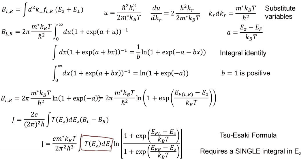
Slide 7: the derivation completed, the Tsu–Esaki formula requiring a single integral in E_z — Slide 7: the substitution, the integral identity, $B_{L,R}$, and the final formula, which "requires a SINGLE integral in $E_z$".

Putting $B_L - B_R$ back into $J$ gives

J = \frac{e\,m^*k_BT}{2\pi^2\hbar^3}\int T(E_z)\, \ln\frac{1 + e^{(\mu_L - E_z)/k_BT}}{1 + e^{(\mu_R - E_z)/k_BT}}\,dE_z .

In open-nemo, Heterostructure1D.current_density(E, T, mu_L, mu_R, temperature) is this formula with the mass of the left contact. The prefactor in practical units: with $m^*/\hbar^2$ in 1/(eV nm$^2$) and $e/\hbar$ in C/(eV s), $e m^*k_BT/(2\pi^2\hbar^3)$ times an energy integral in eV is a current per nm$^2$; one nm$^{-2}$ is $10^{14}$ cm$^{-2}$.

Code30 lines · cell 5

gaas = EM("GaAs", m, 12.9)
algaas = EM("AlGaAs", m, 12.2, conduction_band_edge=0.3)       # equal mass: Tsu-Esaki is exact
layers = [nemo.Layer(mat, w) for mat, w in ((gaas, 10), (algaas, 5), (gaas, 5), (algaas, 5), (gaas, 10))]
dev = nemo.Heterostructure1D(layers, spacing=0.05, mass_average="mean")
x = dev.x
tr = nemo.Transport(dev.hamiltonian)


def linear_drop(v):                     # the bias drops across the 15 nm double barrier (Lecture 10.1)
    return -v * np.clip((x - 10.0) / 15.0, 0.0, 1.0)


def energy_grid(pot, lo, hi, n=4000):
    res = nemo.resonances(dev, potential=pot)
    parts = [np.linspace(lo, hi, n)]
    parts += [e + w * np.linspace(-40, 40, 401) for e, w in zip(res["energy"], res["width"]) if lo < e < hi]
    e = np.unique(np.concatenate(parts))
    return e[(e >= lo) & (e <= hi)]


prefactor = (Q / HBAR) * m_hbar2 * kt / (2 * np.pi**2) * 1e14  # A/cm^2 per eV of the integral
print(f"e m* kT / (2 pi^2 hbar^3) = {prefactor:.4e} A/cm^2 per eV at {T:.0f} K")
v = 0.1
pot = linear_drop(v)
ez = energy_grid(pot, -v + 1e-5, mu + 15 * kt)
t = tr.transmission(ez, potential=pot)
supply = log1p_exp((mu - ez) / kt) - log1p_exp((mu - v - ez) / kt)
j_hand = prefactor * np.trapezoid(t * supply, ez)
j_lib = dev.current_density(ez, t, mu, mu - v, T)
print(f"V = {v} V: hand-coded Tsu-Esaki {j_hand:.2f} A/cm^2, dev.current_density {j_lib:.2f} A/cm^2")

e m* kT / (2 pi^2 hbar^3) = 2.8031e+07 A/cm^2 per eV at 300 K
V = 0.1 V: hand-coded Tsu-Esaki 11573.05 A/cm^2, dev.current_density 11573.05 A/cm^2

The hand-coded formula and the library agree. To see what the formula saves, the next cell evaluates the triple integral directly on the same device: 64 Gauss–Legendre points in $k_r$, and at each one a full $T(E_z, k_\perp)$ calculation on an energy grid refined around that $k$'s resonances, with the transverse energy passed to the 1-D problem as a potential. The time and the number of transmission evaluations are counted for both.

Code23 lines · cell 7

import time

clock = time.perf_counter()
ez = energy_grid(pot, -v + 1e-5, mu + 15 * kt)
j_te = dev.current_density(ez, tr.transmission(ez, potential=pot), mu, mu - v, T)
t_te, n_te = time.perf_counter() - clock, ez.size

clock = time.perf_counter()
k_max = np.sqrt((mu + 15 * kt + v) * m / H2M0)
xg, wg = np.polynomial.legendre.leggauss(64)
kr, wk = 0.5 * k_max * (xg + 1), 0.5 * k_max * wg
total, n_full = 0.0, 0
for k, w in zip(kr, wk):
    pk = pot + H2M0 * k**2 / dev.mass
    e = energy_grid(pk, -v + 1e-5, mu + 15 * kt)
    occ = fermi(e, mu, T) - fermi(e, mu - v, T)            # total energy E = E_z + E_perp
    total += w * k / np.pi * np.trapezoid(tr.transmission(e, potential=pk) * occ, e)
    n_full += e.size
j_full = Q / H * total * 1e14
t_full = time.perf_counter() - clock
print(f"Tsu-Esaki:      J = {j_te:9.2f} A/cm^2, {n_te:6d} transmissions, {t_te * 1e3:6.0f} ms")
print(f"triple integral J = {j_full:9.2f} A/cm^2, {n_full:6d} transmissions, {t_full * 1e3:6.0f} ms")
print(f"ratio {j_full / j_te:.5f}; cost ratio {n_full / n_te:.0f}x in transmissions")

Tsu-Esaki:      J =  11573.05 A/cm^2,   4550 transmissions,     20 ms
triple integral J =  11577.39 A/cm^2, 280816 transmissions,   1182 ms
ratio 1.00037; cost ratio 62x in transmissions

For this equal-mass device the two agree to the accuracy of the quadratures (0.04%), and the triple integral costs 62 times as many transmissions (and about 60 times the time), one resonance search per $k$ included. On a laptop today that is a fraction of a second; in the 1990s, in Klimeck's words, "it was incredibly intense to calculate such things", and the single integral of Tsu and Esaki was what made RTD simulation routine. The price is the assumption $T(E_z, \mathbf k_\perp) = T(E_z)$: Lecture 10.7 showed that a heavier barrier mass alone changes the current of the same structure by up to 18%.

Slide 8: the Tsu–Esaki formula next to the k = 0 calculation it needs — Slide 8: one transmission calculation at $k = 0$ (left) replaces the whole $(E, k)$ family (middle and right).

4. The supply function#

The logarithm in the Tsu–Esaki formula is the difference of two supply functions, $N_{L,R}(E_z) = k_BT\ln(1 + e^{(\mu_{L,R} - E_z)/k_BT})$, the occupied transverse states per $E_z$ in units of the 2-D density of states. The figure shows $N_L$ for $\mu_L = 50$ meV at three temperatures, with its degenerate limit $(\mu_L - E_z)\,\theta(\mu_L - E_z)$, and $N_L - N_R$ at 0.1 V.

Code19 lines · cell 9

e = np.linspace(-0.12, 0.15, 1000)
fig, (a1, a2) = plt.subplots(1, 2, figsize=(11, 3.8))
for temp, c in zip((4.0, 77.0, 300.0), style.sweep(3)):
    kti = KB * temp
    a1.plot(e * 1e3, kti * log1p_exp((mu - e) / kti) * 1e3, color=c, label=f"{temp:.0f} K")
    diff = log1p_exp((mu - e) / kti) - log1p_exp((mu - 0.1 - e) / kti)
    a2.plot(e * 1e3, kti * diff * 1e3, color=c, label=f"{temp:.0f} K")
a1.plot(e * 1e3, np.clip(mu - e, 0, None) * 1e3, "k--", lw=0.8, label="degenerate limit")
a1.set(xlabel="E_z (meV)", ylabel="N_L(E_z) (meV)", title="Supply function, μ_L = 50 meV")
a2.set(xlabel="E_z (meV)", ylabel="N_L − N_R (meV)", title="Supply difference at 0.1 V")
for ax in (a1, a2):
    ax.axvline(mu * 1e3, color=style.CONTEXT, ls=":", lw=0.8)
    ax.legend(frameon=False, fontsize=8)
fig.tight_layout()
for temp in (4.0, 77.0, 300.0):
    kti = KB * temp
    print(f"{temp:5.0f} K: N_L at E_z = 0 is {kti * log1p_exp(mu / kti) * 1e3:6.2f} meV, "
          f"at E_z = mu {kti * np.log(2) * 1e3:6.2f} meV, "
          f"at mu + 50 meV {kti * log1p_exp(-0.05 / kti) * 1e3:.2e} meV")

    4 K: N_L at E_z = 0 is  50.00 meV, at E_z = mu   0.24 meV, at mu + 50 meV 3.47e-64 meV
   77 K: N_L at E_z = 0 is  50.00 meV, at E_z = mu   4.60 meV, at mu + 50 meV 3.54e-03 meV
  300 K: N_L at E_z = 0 is  53.49 meV, at E_z = mu  17.92 meV, at mu + 50 meV 3.49e+00 meV

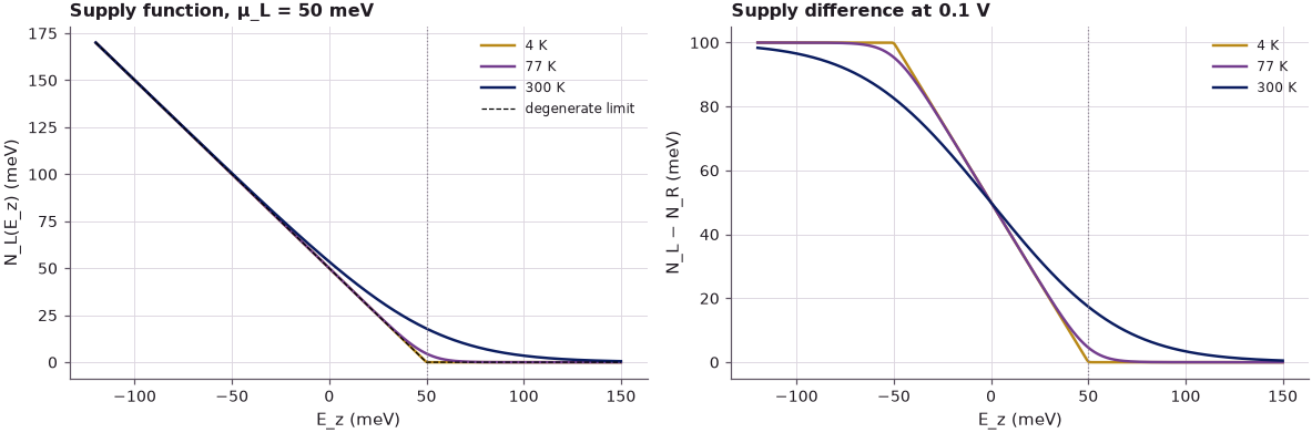
Figure computed by the notebook with open-nemo

At 4 K the supply function is the degenerate triangle: 50 meV of supply at the band edge, falling linearly to zero at $\mu_L$ (it is $k_BT\ln 2 = 0.24$ meV there). At 77 K the triangle is rounded near $\mu_L$ (4.6 meV at $E_z = \mu_L$). At 300 K it is 53.5 meV at the band edge, 17.9 meV at $\mu_L$ and still 3.5 meV at 50 meV above $\mu_L$, so a resonance above the Fermi level carries current. With bias, $N_L - N_R$ is flat at $eV$ wherever both contacts are degenerate (below $\mu_R$, where left- and right-movers cancel except for that difference) and falls to zero above $\mu_L$.

5. The I–V at 4, 77 and 300 K#

With a single resonance of width $\Gamma$ inside the window, at low temperature the integral picks up the supply at the resonance: $J \approx \frac{e m^*}{2\pi^2\hbar^3}\,(\mu_L - E_r)\int T\,dE_z$ while $E_r$ lies between the emitter band edge and $\mu_L$ (and above $\mu_R$). For a Breit–Wigner peak $\int T\,dE_z = (\pi\Gamma/2)\,T_\text{peak}$, with $T_\text{peak} = 4\Gamma_L\Gamma_R/(\Gamma_L + \Gamma_R)^2$ equal to 1 only for equally transparent barriers (Lecture 10.3). If $\int T$ stayed constant, the current would grow linearly as the bias pulls $E_r$ down and drop to nearly zero once $E_r$ passes below the emitter band edge: the triangular I–V of an ideal RTD. The table below the figure compares the 4 K current with this estimate, using the numerical $\int T\,dE_z$ over $\pm 40\Gamma$ around the resonance.

Code35 lines · cell 11

biases = np.linspace(0.0, 0.3, 61)
iv = {}
for temp in (4.0, 77.0, 300.0):
    kti = KB * temp
    j = []
    for vb in biases:
        p = linear_drop(vb)
        egrid = energy_grid(p, -vb + 1e-5, mu + 20 * kti)
        j.append(dev.current_density(egrid, tr.transmission(egrid, potential=p), mu, mu - vb, temp))
    iv[temp] = np.array(j)

fig, ax = plt.subplots(figsize=(6.2, 3.9))
for (temp, j), c in zip(iv.items(), style.sweep(3)):
    ax.plot(biases, j / 1e3, "o-", ms=2.5, color=c, label=f"{temp:.0f} K")
ax.set(xlabel="Bias (V)", ylabel="Current density (kA/cm²)", title="Tsu–Esaki I–V of the double barrier")
ax.legend(frameon=False, fontsize=8)

pref0 = Q / HBAR * m_hbar2 / (2 * np.pi**2) * 1e14            # e m*/(2 pi^2 hbar^3), A/cm^2 per eV^2
print("  V (V)   E_r (meV)  Gamma (meV)  T_peak  int T dE (meV)   4 K numeric   estimate (A/cm^2)")
for vb in (0.06, 0.08, 0.10, 0.12, 0.14, 0.16):
    p = linear_drop(vb)
    rr = nemo.resonances(dev, potential=p)
    er, gv = rr["energy"][0], rr["width"][0]
    eres = er + gv * np.linspace(-40, 40, 4001)
    tres = tr.transmission(eres, potential=p)
    area = np.trapezoid(tres, eres)
    est = pref0 * max(mu - er, 0.0) * area
    j4 = iv[4.0][np.argmin(abs(biases - vb))]
    print(f"  {vb:.2f}    {er * 1e3:7.2f}    {gv * 1e3:6.3f}    {tres.max():.3f}    {area * 1e3:7.4f}"
          f"      {j4:9.1f}       {est:9.1f}")
cross = biases[np.argmax([nemo.resonances(dev, potential=linear_drop(vb))["energy"][0] < 0 for vb in biases])]
print(f"the resonance passes the emitter band edge between {cross - 0.005:.3f} and {cross:.3f} V")
for temp, j in iv.items():
    ip = int(np.argmax(j))
    print(f"{temp:5.0f} K: peak {j[ip]:8.1f} A/cm^2 at {biases[ip]:.3f} V, valley {j[ip:].min():7.1f} A/cm^2")

  V (V)   E_r (meV)  Gamma (meV)  T_peak  int T dE (meV)   4 K numeric   estimate (A/cm^2)
  0.06      59.32     0.444    0.822     0.5705           10.5             0.0
  0.08      49.16     0.466    0.705     0.5137          547.7           466.2
  0.10      38.96     0.495    0.576     0.4458         5275.5          5336.6
  0.12      28.71     0.530    0.445     0.3686         8428.0          8508.2
  0.14      18.42     0.571    0.315     0.2816         9564.6          9645.4
  0.16       8.08     0.616    0.183     0.1771         7978.4          8051.1
the resonance passes the emitter band edge between 0.175 and 0.180 V
    4 K: peak   9564.6 A/cm^2 at 0.140 V, valley   102.9 A/cm^2
   77 K: peak   9590.9 A/cm^2 at 0.140 V, valley   118.0 A/cm^2
  300 K: peak  12601.4 A/cm^2 at 0.125 V, valley  1619.4 A/cm^2

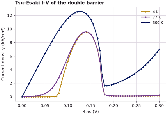
At 4 K the estimate $(\mu_L - E_r)\,e m^*\!\int T\,dE_z/(2\pi^2\hbar^3)$ reproduces the numerical current to within 1% from 0.10 to 0.16 V; at 0.08 V, where the resonance sits only 0.8 meV below $\mu_L$, it is 15% low. The table also shows why the I–V is not the ideal triangle: the linear drop makes the two barriers unequally transparent, the peak transmission falls from 0.82 at 0.06 V to 0.18 at 0.16 V, and $\int T\,dE_z$ falls with it. The current therefore peaks at 0.14 V (9.56 kA/cm$^2$), before the resonance reaches the emitter band edge between 0.175 and 0.180 V, and then collapses to about 0.1 kA/cm$^2$. At 77 K the I–V hardly changes (peak 9.59 kA/cm$^2$ at 0.14 V) apart from a softer onset. At 300 K the current starts at zero bias, because the Boltzmann tail of the supply reaches the resonance above $\mu_L$; the peak rises to 12.6 kA/cm$^2$ at 0.125 V and the valley is 1.6 kA/cm$^2$, carried by the thermal tail at higher energies. Lecture 10.1 showed the same physics with a 1-D Landauer current, without the transverse supply.

Summary#

The 3-D Landauer formula for a layered device is a triple integral over $E_z$ and $\mathbf k_\perp$; with $T(E_z, \mathbf k_\perp) = T(E_z)$ and cylindrical symmetry the transverse integral is analytic.
The transverse kernel $B = (2\pi m^*k_BT/\hbar^2)\ln(1 + e^{(\mu - E_z)/k_BT})$ matches a brute-force $(k_x, k_y)$ sum to six digits; the identity behind it holds to ten.
The hand-coded Tsu–Esaki formula agrees with dev.current_density; for an equal-mass device it agrees with the full triple integral to 0.04% at 1/62 of the transmission evaluations.
The supply function $k_BT\ln(1 + e^{(\mu - E_z)/k_BT})$ is a triangle at low temperature and has a Boltzmann tail at 300 K. At 4 K the current follows $(\mu_L - E_r)\,e m^*\!\int T\,dE_z/(2\pi^2\hbar^3)$ to 1%, and the falling peak transmission under bias moves the peak (9.56 kA/cm$^2$ at 0.14 V) ahead of the point where the resonance leaves the emitter band (0.175–0.180 V).

Exercises#

Derive the degenerate limit of the Tsu–Esaki formula at $T = 0$ and show that for $eV < \mu_L$ it gives $J = \frac{e m^*}{2\pi^2\hbar^3}\left[eV\int_0^{\mu_R}T\,dE_z + \int_{\mu_R}^{\mu_L}(\mu_L - E_z)T\,dE_z\right]$. Check it against the 4 K curve.
Use a right contact with a different mass (an InGaAs collector, say $m^* = 0.041\,m_0$) and compare current_density (which uses the left contact's mass for both sides) with the triple integral of Section 3. Which assumption of slide 4 is broken?
Replace the Fermi–Dirac occupation by a Boltzmann factor in $B$. For which $E_z$ is the error larger than 10% at 300 K with $\mu_L = 50$ meV?