The recursive Green function algorithm (RGF)

1. What NEGF has to compute#

This lecture is about numerics: how the Green functions used in all RTD calculations of this section are actually obtained. Two quantities are needed.

Dynamics, the states of the system. The retarded Green function solves

where \(E\) is the energy (eV), \(H\) the device Hamiltonian, \(\Sigma^R_\text{bound} = \Sigma^R_\text{left} + \Sigma^R_\text{right}\) the self-energies that describe escape into the contacts and \(\Sigma^R_\text{scatt}\) the escape into other channels by scattering. \(G^R\) is the impulse response of the device: it tells where electrons can be.

Kinetics, the occupation. The lesser Green function counts the electrons,

with \(\Gamma = i(\Sigma^R - \Sigma^{R\dagger})\) the broadening of a contact and \(f\) its Fermi function. The lecture's analogy: \(G^R\) is the set of apartments, \(G^<\) tells which apartments are occupied. Here scattering is left out (\(\Sigma_\text{scatt} = 0\)); it is the subject of lecture 13. For a full course on NEGF the lecture recommends Supriyo Datta's lectures on nanoHUB.

The device is split into three domains: a left reservoir, the central device (sites \(0 \dots N-1\)) and a right reservoir. Each reservoir is a semi-infinite lead. Its left-connected Green function \(g^R_{-1,-1}\) on the last lead site knows everything about the lead from site \(-1\) to \(-\infty\); coupled into the device by the hopping \(t_{-1,0}\) it gives the boundary self-energy on site 0,

and the same on site \(N-1\) from the right lead. For a single-band lead with hopping \(t\) and band bottom \(E_c\) this is analytic, \(\Sigma^R = -t\,e^{ika}\) with \(\cos ka = 1 - (E - E_c)/2t\); for multiband leads it is computed numerically, for example with the Sancho–Rubio iteration.

The test device is the RTD of lecture 11.1: GaAs contacts, two 5 nm Al${0.3}$Ga${0.7}$As barriers and a 7 nm GaAs well, discretised with \(a = 0.1\) nm. Its Hamiltonian is a tridiagonal matrix with on-site energies \(\varepsilon_i\) and hoppings \(-t_i\), \(t = \hbar^2/(2 m^* a^2)\); rtd.lead_self_energy returns the analytic lead self-energy.

2. \(G^R\) is a full matrix, and inverting it is expensive#

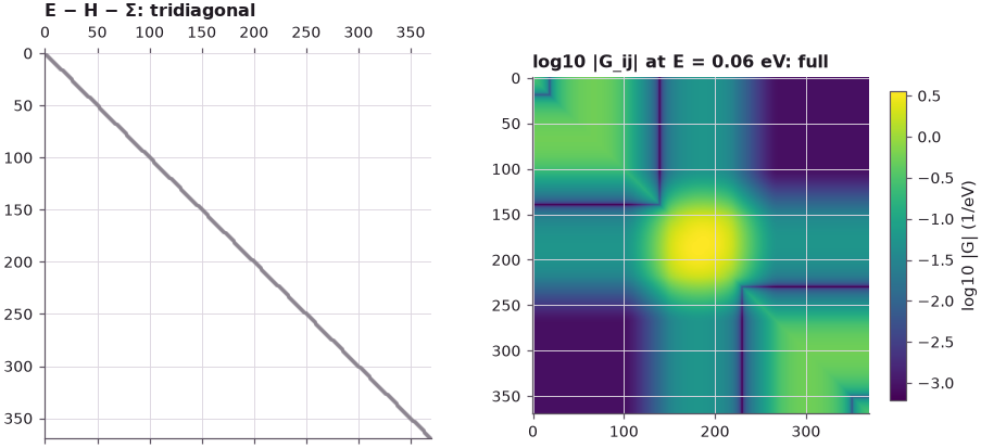
\(E - H - \Sigma^R\) is tridiagonal; only the two corner sites are modified by the self-energies. Its inverse, however, is a full matrix: an impulse on any site reaches every other site. The figure shows \(|G^R_{ij}|\) at an energy just above the first resonance.

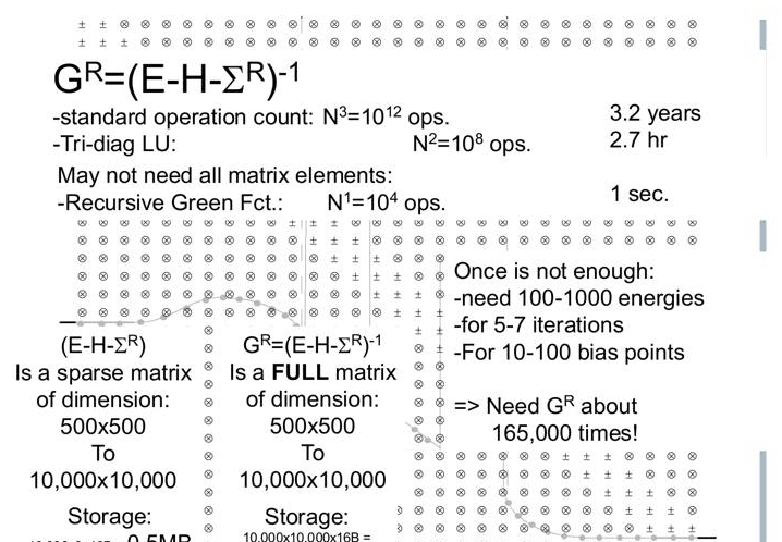
The lecture counts the cost for a realistic device. An RTD with 100 nm contacts and 5 nm barriers and well has 500 to 1000 sites; in a multiband tight-binding model each site is a \(10\times10\) or \(20\times20\) block, so the matrix order is between 500 and 10 000. A full inversion costs \(\sim N^3\) operations, a tridiagonal LU factorisation that produces the whole inverse \(\sim N^2\), and the recursive algorithm \(\sim N\). Storage follows the same logic: the sparse matrix needs about \(3N\) complex numbers, the full \(G^R\) needs \(N^2\).

3. Which elements are needed?#

Without incoherent scattering, only a few elements of \(G^R\) enter the observables:

• Current only (the charge comes from a semiclassical model, as in the Thomas–Fermi calculations of lectures 11.1–11.3): the transmission is \(T(E) = \Gamma_L \Gamma_R |G^R_{0,N-1}|^2\), one single element.
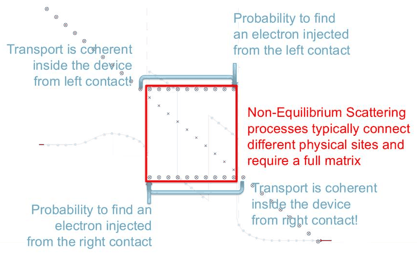
• Current and charge (Hartree, lecture 11.4): the electron density on site \(i\) needs the diagonal of \(G^< = G^R \Sigma^< G^{R\dagger}\), that is \(\Gamma_L |G^R_{i,0}|^2 f_L + \Gamma_R |G^R_{i,N-1}|^2 f_R\) in the non-equilibrium region, the first and last columns of \(G^R\); in the reservoirs, where the occupation is an equilibrium one, the diagonal \(G^R_{i,i}\) suffices.

The two columns have a direct meaning: \(\Gamma_L |G^R_{i,0}|^2/2\pi\) is the probability density of finding on site \(i\) an electron injected from the left contact, \(\Gamma_R |G^R_{i,N-1}|^2/2\pi\) the same for an electron from the right contact. Their sum is the local density of states \(-\operatorname{Im} G^R_{ii}/\pi\).

4. The recursions#

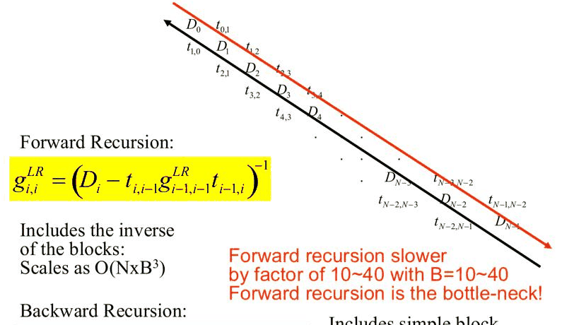
Write the matrix to be inverted as \(A = E - H - \Sigma^R\) with diagonal blocks \(D_i\) (here numbers, \(D_i = E - \varepsilon_i - \Sigma_i\)) and off-diagonal blocks \(t_{i,i\pm1}\), the off-diagonal entries of \(A\) (here \(t_{i,i+1} = -H_{i,i+1}\)).

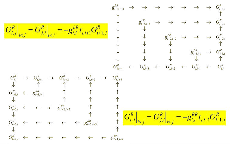
Forward recursion (left-connected Green functions). \(g^{L}_{i,i}\) is the Green function of site \(i\) with everything to its left connected and everything to its right cut off:

The last one, \(g^L_{N-1,N-1}\), includes the right lead through \(D_{N-1}\) and is therefore the exact element \(G^R_{N-1,N-1}\): left-connected and right-connected meet at the last site.

Backward recursion (diagonal of \(G^R\)):

Off-diagonal elements, by walking from the diagonal one step at a time:

which gives the last column \(G^R_{i,N-1}\) from \(G^R_{N-1,N-1}\). For the current alone, the corner element can be carried along in the forward pass: the left-connected corner element obeys \(g^{L}_{0,i} = -\,g^{L}_{0,i-1}\, t_{i-1,i}\, g^{L}_{i,i}\), and \(G^R_{0,N-1} = g^L_{0,N-1}\). The first column follows from the same recursions run from the right (right-connected Green functions).

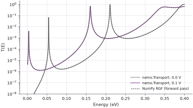
The RGF elements agree with the dense inverse to round-off. Now the transmission through the RTD, \(T(E) = \Gamma_L \Gamma_R |G^R_{0,N-1}|^2\) from the forward pass alone, against nemo.Transport (open-nemo's own RGF implementation), at zero bias and with a linear drop of 0.1 V across the barriers and the well.

5. What the matrix elements mean#

With the diagonal and the two columns, the local density of states and the left- and right-injected spectral functions follow on every site:

The map shows the LDOS of the unbiased RTD; the line plots the left- and right-injected spectral functions at the first resonance with the 0.1 V drop of lecture 11.1 applied (from 10 to 27 nm).

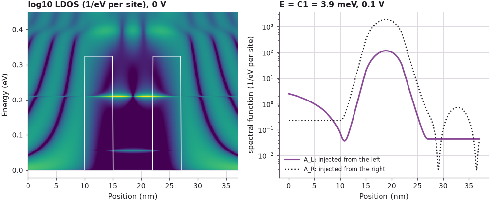
The LDOS map shows the quasi-bound states in the well as bright lines and the standing-wave patterns of the contact states reflected by the barriers. The sum rule holds to round-off. At 0.1 V the resonance C1 lies only 3.9 meV above the emitter band edge: electrons arriving from the left have very little kinetic energy there and couple weakly to the well, while from the collector side, more than 0.1 eV above its band edge, the coupling is much stronger, so \(A^R\) is 16 times larger than \(A^L\) in the well. Which of the two actually holds electrons is decided by the Fermi functions: the collector states at this energy are empty, its Fermi level being 0.1 eV lower, so the charge in the well comes from \(A^L f_L\) alone. This is the physics behind the off-diagonal strips of slide 22: the first column of \(G^R\) carries what the left contact injects, the last column what the right contact injects, and each is weighted with its own Fermi function.

6. Cost against the number of sites#

The following cell times one energy point for chains of increasing length: the dense inverse (\(N^3\)), the banded (tridiagonal) LU solve for the whole inverse (\(N^2\)), the NumPy RGF with the full backward pass and with the forward pass only (\(N\)), and nemo.Transport. All timings use one BLAS thread.

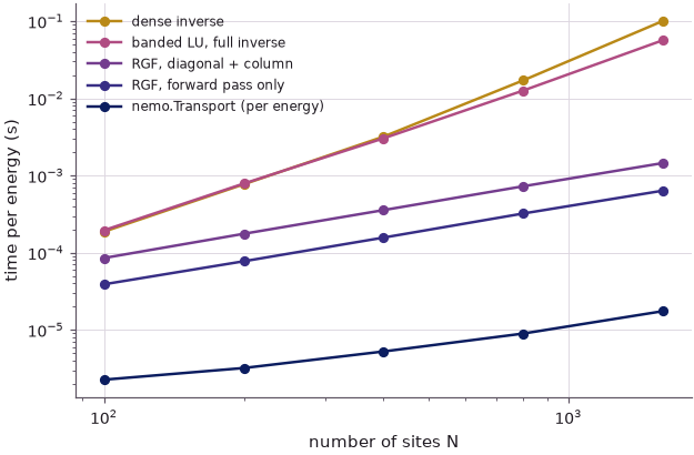
The fitted slopes of the log–log curves over the three largest sizes are printed (timings vary by a few per cent from run to run). The dense inverse grows with a slope of about 2.5 (LAPACK is very efficient at these moderate sizes, so the slope is still below the asymptotic 3), the banded LU solve that produces all \(N^2\) elements with a slope of about 2.1, and both RGF variants linearly. At 1600 sites the dense inverse takes about 100 ms per energy and the NumPy forward pass about 0.65 ms, more than 100 times less. The NumPy loop has a large constant cost per site from the Python interpreter; the compiled implementation in nemo.Transport needs about 0.016 ms per energy at the same size (its slope of about 0.8 still contains a fixed cost per call). The ratio between dense and recursive solutions grows without bound with \(N\), which is the payoff the lecture describes: years of computing reduced to seconds.

7. Block tridiagonal matrices: \(O(N B^3)\)#

In a multiband or multi-dimensional model each site (or layer) is a block of size \(B\): \(D_i\) and \(t_{i,i+1}\) become \(B\times B\) matrices and the scalar divisions become block inversions. The same code with matrix operations handles, for example, a 2D strip of width \(B\) sites on a square lattice (hopping 1 eV, arbitrary units), whose leads are strips of the same width. 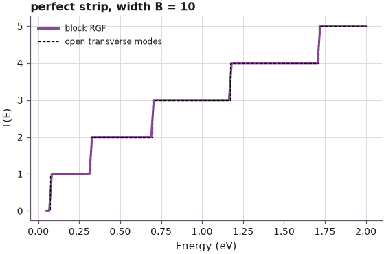The lead self-energies come from open-nemo's Sancho–Rubio solver, nemo.solvers.transport.self_energy. In a perfect strip the transmission must count the open transverse modes, an integer staircase.

The cost of the block recursion is \(N\) block inversions and multiplications of \(B\times B\) matrices, \(O(N B^3)\), against \(O((NB)^3)\) for a dense inversion of the whole matrix of order \(NB\). The timing below uses 40 slabs and widths from 5 to 80.

Both methods give the same diagonal blocks to round-off. At small \(B\) the block recursion is dominated by Python overhead per slab, so its time hardly grows; at large \(B\) the block operations dominate and the growth steepens (a slope of about 2 between \(B = 40\) and 80, where optimised small-matrix BLAS still hides part of the \(B^3\)), while the dense inverse grows with a slope near 2.8 and at \(B = 80\) is about 60 times slower. In operation count the dense inversion of the order-\(NB\) matrix is \(N^2 = 40^2\) times more expensive than the \(N\) block inversions. This is the \(O(N B^3)\) scaling of slide 35, and the reason the lecture names the forward recursion, which contains the block inversions, as the bottleneck.

8. Scattering fills the matrix#

Everything above relied on \(E - H - \Sigma\) being (block) tridiagonal. A boundary self-energy only touches the two end blocks. Incoherent scattering adds \(\Sigma^R_\text{scatt} = D \times G^R\): if the scattering is local (an interaction that only couples a site to itself, such as a deformation-potential or Büttiker-probe model), \(\Sigma_\text{scatt}\) is diagonal and the recursions still apply, inside a self-consistent loop. A non-local interaction, in which an electron on one site feels a lattice vibration or a charge further away (polar optical phonons, Coulomb scattering), couples distant sites, makes \(\Sigma_\text{scatt}\) and therefore \(E - H - \Sigma\) full, and the recursive algorithm loses its advantage. Practical codes then restrict the full treatment to a small central region, which is the strategy of the NEMO "central region with reservoirs" partitioning used in lectures 11.3 and 13.

Summary#

• NEGF needs the retarded Green function \(G^R = (E - H - \Sigma^R)^{-1}\) (the states) and the lesser Green function \(G^< = G^R \Sigma^< G^{R\dagger}\) (their occupation). The leads enter through boundary self-energies on the first and last site, computed from left- and right-connected lead Green functions.
• \(E - H - \Sigma\) is tridiagonal but \(G^R\) is full. A full inversion costs \(N^3\) operations, a tridiagonal LU for the whole inverse \(N^2\), and the recursive algorithm \(N\) (for blocks of size \(B\): \(N B^3\)).
• The current needs a single element \(G^R_{0,N-1}\), available after the forward pass; the charge needs the diagonal (equilibrium reservoirs) and the first and last columns (non-equilibrium region).
• The forward recursion builds left-connected Green functions, the backward recursion the diagonal of \(G^R\), and a further recursion walks to off-diagonal elements. In the NumPy implementation here all elements agree with the dense inverse to round-off and the transmission agrees with nemo.Transport.
• Local scattering keeps the matrix tridiagonal; non-local scattering fills it and requires full-matrix methods on a reduced central region.

Exercises#

1. Modify rgf to return the nearest off-diagonal elements \(G^R_{i,i+1}\) and use them to compute the current density between sites \(i\) and \(i+1\) at the resonance energy. Check that it is the same on every bond (current conservation).
2. Integrate \(A^L_i f_L + A^R_i f_R\) over energy at 0.1 V and 77 K to obtain the electron density along the RTD, and compare it with the semiclassical density of the contacts.
3. Time rgf and rgf_block with B = 1 for the same chain. How much of the per-site cost is Python overhead, and how would you reduce it?
4. Add a constant imaginary part \(-i\eta\) to all \(D_i\) (a crude local scattering model, \(\eta = 1\) meV) and check that the RGF still agrees with the dense inverse. What happens to the sum rule \(A^L + A^R = -2\operatorname{Im} G^R_{ii}\), and why?

Further reading#

• Lecture 11.5: asymmetric RTDs
• Lecture 13: incoherent scattering in RTDs
• Green functions from scratch: self-energies, transmission and RGF timing
• Bound states in open devices
• Lake et al. 1997: multiband NEGF for RTDs
• Lecture slides 2–48, in particular slides 26–36 (the recursions step by step) and slide 47 (equation summary).
• R. Lake, G. Klimeck, R. C. Bowen and D. Jovanovic, J. Appl. Phys. 81, 7845 (1997).
• M. P. Lopez Sancho, J. M. Lopez Sancho and J. Rubio, J. Phys. F 15, 851 (1985).
• S. Datta, Quantum Transport: Atom to Transistor (Cambridge University Press, 2005).