

Lecture 20
Introduction to quantum dots
In the lecture
- What a quantum dot is: a small low-energy region enclosed in all three directions, an "artificial atom" with quantized levels and a countable number of electrons.
- The wavefunctions of a pyramidal self-assembled dot, whose shape breaks the cubic symmetry.
- Three ways to make dots (self-assembled epitaxy, electrostatic gates, colloidal chemistry) and the applications foreseen around 1998: logic, memory, single-electron transistors, markers, infrared detectors, quantum computing.
- Why dots absorb normally incident infrared light that a quantum well cannot.
- Size as the colour knob: colloidal CdSe dots in displays, colour gamut, and the 2023 Nobel Prize in Chemistry.
- Single electronics: when the charging energy \(e^2/2C\) exceeds \(k_BT\).
In this notebook
- Solve the effective-mass Schrödinger equation of a pyramidal InGaAs-like dot on a 3-D grid with open-nemo, plot its s- and p-like states and compute their optical dipole matrix elements, which show why dots respond to light polarised in the growth plane.
- Compute the band gap of passivated spherical CdSe nanocrystals of 2 to 5 nm diameter with sp3d5s* tight binding, convert it to an emission wavelength and compare with the size–colour table of the lecture and with the effective-mass (Brus) formula.
- Compare the charging energy of a dot with \(k_BT\) to see which sizes and temperatures allow single-electron operation.
Run it on your own machine
The notebook needs open-nemo (Python ≥ 3.10 and a C++20 compiler; BLAS/LAPACK).
git clone https://github.com/denphi/open-nemo.git && cd open-nemo
python3 -m venv .venv && source .venv/bin/activate
pip install -e ".[notebooks]"
jupyter lab From_Atoms_to_Devices/07_quantum_dots_and_nemo3d/20_0_introduction_to_quantum_dots.ipynbCode
import time
import numpy as np
import matplotlib.pyplot as plt
import opennemo as nemo
from opennemo.visualization import style
from opennemo.structures.structure import Structure, cluster, bulk
from opennemo.structures.shapes import Sphere
from opennemo.core import units

style.use(notebook=True)
H2M = units.HBAR2_2M0          # hbar^2 / (2 m0) = 0.0381 eV nm^2
1. What is a quantum dot?#
A quantum dot is a region of low electron energy (a small-gap or well-conducting material) that is surrounded in all three dimensions by a region of higher energy (a wide-gap or poorly conducting material). Three conditions make it behave as a dot rather than as a small piece of bulk:
- its size is a few nanometres, comparable to the electron wavelength, so that the energies are quantized;
- decoherence is weak: the length over which an electron keeps its phase is larger than the dot;
- it then holds a countable number of electrons in discrete levels, like an atom. Klimeck calls it an artificial atom; several dots close to each other form an artificial molecule.
The lecture lists three ways to use such states: absorb photons (detectors, inputs), emit photons (lasers, LEDs, outputs), and move or store charge by tunneling into the levels (logic and memory).
The simplest model of confinement is a particle in a box with infinite walls, of side lengths \(L_x, L_y, L_z\):
with \(m^*\) the effective mass. In a cube the levels (2,1,1), (1,2,1), (1,1,2) are threefold degenerate. A real self-assembled dot is not a cube.
2. Wavefunctions of a pyramidal dot#
Self-assembled InGaAs dots grown on GaAs (the lecture shows images by Rosa Leon, JPL, 1998) are pyramids or domes, wide and flat: about 20 nm across and a few nanometres tall. Their shape breaks the cubic symmetry of the box. The ground state is s-like; the next two states have one node along \(x\) or along \(y\) (p$_x$, p$_y$) and stay degenerate because the square base keeps the \(x\) and \(y\) directions equivalent; a state with a node along \(z\) (p$_z$) costs much more energy because the dot is thin, and it looks different from p$_x$ and p$_y$.

Here the same physics is computed in the single-band effective-mass model: a pyramid with a 20 nm square base and 7 nm height, on a 0.75 nm thick wetting layer, inside a barrier 0.5 eV higher, with \(m^* = 0.05\,m_0\). The Hamiltonian is a 7-point finite-difference Laplacian on a cubic grid of spacing \(h = 0.75\) nm, built by open-nemo as a one-orbital tight-binding model with on-site energy \(6t\) and hopping \(-t\), where \(t = \hbar^2/(2m^*h^2)\); the confinement enters as an on-site potential.
Code
MSTAR, BARRIER, h = 0.05, 0.5, 0.75          # m*/m0, band offset (eV), grid spacing (nm)
BASE, HEIGHT = 20.0, 7.0                     # pyramid base and height (nm)
t_hop = H2M / (MSTAR * h * h)                # hopping energy t (eV)
nx, nz = 40, 24                              # 30 x 30 x 18 nm box
grid = np.stack(np.meshgrid(np.arange(nx) * h, np.arange(nx) * h, np.arange(nz) * h,
                            indexing="ij"), -1).reshape(-1, 3)
box = Structure(grid, ["X"] * len(grid), np.diag([nx * h, nx * h, nz * h]))
fd = nemo.models.tb.single_band_material(h, onsite=6 * t_hop, hopping=-t_hop)
h_grid = nemo.models.tb.SlaterKoster(fd).build(box)

centre = np.array([nx * h / 2, nx * h / 2, 5.0])     # centre of the pyramid base
rel = grid - centre
half = BASE / 2 * (1 - rel[:, 2] / HEIGHT)           # half-width of the pyramid at height z
in_pyr = (rel[:, 2] >= 0) & (rel[:, 2] <= HEIGHT) & (np.abs(rel[:, 0]) <= half) & (np.abs(rel[:, 1]) <= half)
wetting = (rel[:, 2] < 0) & (rel[:, 2] >= -h)
u = np.where(in_pyr | wetting, 0.0, BARRIER)

t0 = time.perf_counter()
res = nemo.eigenstates(h_grid, num=8, k=np.zeros(3), potential=u)
order = np.argsort(res["energies"])
E_pyr, psi = res["energies"][order], res["vectors"][:, order]
print(f"{len(grid)} grid points, t = {t_hop:.3f} eV, solved in {time.perf_counter() - t0:.1f} s")
for i, e in enumerate(E_pyr):
    w = np.sum(np.abs(psi[in_pyr | wetting, i])**2)
    print(f"state {i}: E = {e:.4f} eV   probability inside dot = {w:.2f}")
38400 grid points, t = 1.355 eV, solved in 0.8 s
state 0: E = 0.1681 eV   probability inside dot = 0.91
state 1: E = 0.2534 eV   probability inside dot = 0.85
state 2: E = 0.2534 eV   probability inside dot = 0.85
state 3: E = 0.3234 eV   probability inside dot = 0.80
state 4: E = 0.3310 eV   probability inside dot = 0.78
state 5: E = 0.3598 eV   probability inside dot = 0.76
state 6: E = 0.4067 eV   probability inside dot = 0.70
state 7: E = 0.4067 eV   probability inside dot = 0.70
Code
dens = (np.abs(psi)**2).reshape(nx, nx, nz, -1)
iz = int(round((centre[2] + 1.5) / h))               # plane 1.5 nm above the base
iy = nx // 2
ext_xy = [0, nx * h, 0, nx * h]
ext_xz = [0, nx * h, 0, nz * h]
show = [0, 1, 3, 4]
fig, axs = plt.subplots(2, 4, figsize=(12, 5.2))
for j, i in enumerate(show):
    axs[0, j].imshow(dens[:, :, iz, i].T, origin="lower", extent=ext_xy, cmap=style.MAGNITUDE)
    axs[0, j].set(title=f"state {i}: {E_pyr[i]:.3f} eV", xlabel="x (nm)", ylabel="y (nm)")
    axs[1, j].imshow(dens[:, iy, :, i].T, origin="lower", extent=ext_xz, cmap=style.MAGNITUDE)
    axs[1, j].set(xlabel="x (nm)", ylabel="z (nm)")
    axs[0, j].grid(False); axs[1, j].grid(False)
fig.suptitle("|ψ|² of a pyramidal dot: top row x–y plane 1.5 nm above the base, bottom row x–z plane")
fig.tight_layout()
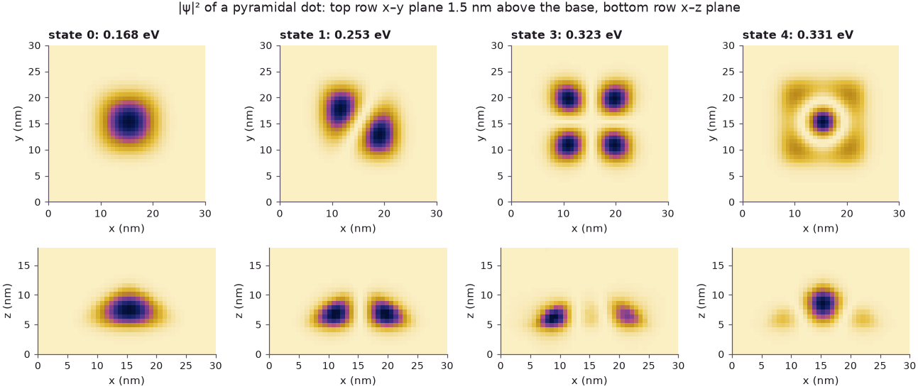
The ground state (state 0) is a single lobe near the base, where the pyramid is widest. States 1 and 2 are degenerate (only state 1 is drawn; state 2 is the same rotated by 90°): a p-like pair with one node in the plane. State 3 has one node along \(x\) and one along \(y\) (four lobes, the "2-2-1" state of slide 3). State 4 is the first state excited along \(z\): its main lobe sits higher in the pyramid, surrounded by a ring near the base. Because the pyramid narrows with height, the vertical and lateral motions do not separate, and this "p$_z$" state looks quite unlike p$_x$ and p$_y$, as the lecture points out; it lies 163 meV above the ground state because the dot is only 7 nm tall. The fraction of probability inside the dot (pyramid plus wetting layer) falls from 0.91 for the ground state to 0.70 for state 6, as the higher states spread into the barrier. The Quantum Dot Lab notebook reproduces the nanoHUB tool the lecturer refers to for 3-D renderings of such states.
3. Ways of making dots and the applications foreseen in 1998#

- Self-assembled dots form during epitaxial growth of InGaAs on GaAs: the larger InAs lattice constant makes the strained film break up into islands. These dots, and their simulation with NEMO 3-D, are the subject of the rest of this section of the course.
- Electrostatic dots: metal or MOS gates on top of a sheet of electrons pinch off a small region.
- Colloidal dots are grown in a chemical solution.
The applications discussed around 1998 were logic with electrostatically coupled dots (quantum cellular automata of Lent and Porod at Notre Dame), room-temperature single-electron transistors (Stanford) and memories (Chou at Princeton, a 128 Mbit integration demonstration by Hitachi), optical markers attached to tissue, quantum computing with charge, spin or optical states (later lectures treat phosphorus donors in silicon), and infrared detectors.
Normal-incidence infrared detection#
An intersubband detector built from a GaAs/AlGaAs quantum well is blind to light that arrives perpendicular to the wafer. In the well the states are \(\psi_n(z)\,e^{i\mathbf{k}_\parallel\cdot \mathbf{r}_\parallel}\), and the dipole matrix element between subbands \(n \neq m\) with polarization in the plane vanishes,
so only the field component along the growth axis \(z\) is absorbed. Light from the top has its electric field in the plane, and a grating is needed to turn the field. A dot is confined in all three directions, so transitions from the s-like ground state to the p$_x$ and p$_y$ states are driven by in-plane fields, and the absorption depends only weakly on the incidence angle.

The dipole matrix elements \(|\langle 0|x|i\rangle|^2\), \(|\langle 0|y|i\rangle|^2\), \(|\langle 0|z|i\rangle|^2\) of the computed pyramid show this directly:
Code
print(f"{'state':>5s} {'E_i - E_0 (meV)':>16s} {'|<0|x|i>|^2':>12s} {'|<0|y|i>|^2':>12s} "
      f"{'|<0|z|i>|^2':>12s}   (nm^2)")
for i in range(1, len(E_pyr)):
    d2 = [abs(np.vdot(psi[:, 0], rel[:, a] * psi[:, i]))**2 for a in range(3)]
    print(f"{i:5d} {1000 * (E_pyr[i] - E_pyr[0]):16.1f} {d2[0]:12.3f} {d2[1]:12.3f} {d2[2]:12.3f}")
pair_xy = sum(abs(np.vdot(psi[:, 0], rel[:, a] * psi[:, i]))**2 for a in (0, 1) for i in (1, 2))
print(f"in-plane strength of the s -> p pair: {pair_xy:.2f} nm^2")
state  E_i - E_0 (meV)  |<0|x|i>|^2  |<0|y|i>|^2  |<0|z|i>|^2   (nm^2)
    1             85.3        6.794        1.859        0.000
    2             85.3        1.859        6.794        0.000
    3            155.4        0.000        0.000        0.000
    4            162.9        0.000        0.000        0.567
    5            191.7        0.000        0.000        0.000
    6            238.6        0.011        0.000        0.000
    7            238.6        0.000        0.011        0.000
in-plane strength of the s -> p pair: 17.31 nm^2
The s→p pair (states 1 and 2, about 85 meV above the ground state, a mid-infrared photon of about 15 µm wavelength) has a large in-plane dipole, \(|x|^2+|y|^2 = 8.65\) nm² for each state of the pair (17.31 nm² for the two together), and none along \(z\). The degenerate pair can come out of the solver as any rotation of p$_x$ and p$_y$, which is why each state shows both an \(x\) and a \(y\) component; the sum is what matters. The first state with a \(z\) node (state 4) couples to \(z\)-polarized light only. A light beam at normal incidence therefore drives the s→p transition of a dot, which a quantum well cannot do.
4. Size is the colour knob: colloidal dots in displays#
The application that took off is light emission. In a colloidal nanocrystal the band gap grows as the size shrinks, so one chemistry (CdSe or InP) covers the whole visible spectrum and only the diameter changes. The lecture's table: about 2 nm emits at 450 nm (blue), 2.8 nm at 510 nm (green), 3.6 nm at 560 nm (yellow), 5 nm at 600 nm (orange) and 6.5 nm at 640 nm (red). The differences in size are small, so size and purity must be well controlled; the reward is a narrow emission line of about 25 nm width, i.e. pure red and green primaries.
In displays, dots are used in three ways: a blue LED backlight shines through a red and green dot film in front of liquid-crystal shutters (QD-LCD, sold as "QLED" since 2013); a blue OLED layer is converted to red and green by dots (QD-OLED); or the dots are driven by current directly (QDEL, the research frontier).

The gamut is the fraction of the colours the eye can see that a screen can make; Rec. 2020 is the reference set for ultra-high-definition video. Colours outside the gamut are clipped to the nearest colour the panel can make: saturated reds become brick, greens olive, cyans slate.
Band gap of CdSe nanocrystals from tight binding#
The dots here are spheres cut from zincblende CdSe (lattice constant 0.608 nm, sp3d5s* parameters
of the nemo5_iivi_sp3d5s set, without spin–orbit coupling), with the dangling bonds of the surface
atoms passivated (moved 30 eV away from the gap). For each diameter the lowest conduction state and
the highest valence state are found by shift-invert Lanczos around two separate reference energies,
near the bulk conduction-band minimum and valence-band maximum; one reference in the middle of the
gap would return surface or deep valence states instead.
Code
cdse = nemo.structures.materials.load("nemo5_iivi_sp3d5s")["CdSe"]
lat = nemo.structures.lattice.from_material(cdse)
e_bulk = np.linalg.eigvalsh(nemo.models.tb.SlaterKoster(cdse).build(bulk(lat)).dense(np.zeros(3)))
EV_BULK = e_bulk[e_bulk < 1.0].max()
EC_BULK = e_bulk[e_bulk > 1.0].min()
print(f"bulk CdSe (TB, Gamma): VBM {EV_BULK:.3f} eV, CBM {EC_BULK:.3f} eV, gap {EC_BULK - EV_BULK:.3f} eV")

diam = np.array([2.0, 2.8, 3.6, 4.4, 5.0])           # nm
gap_tb, n_atoms = [], []
for d in diam:
    t0 = time.perf_counter()
    dot = cluster(lat, Sphere([0.05, 0.07, 0.03], d / 2))
    hdot = nemo.models.tb.SlaterKoster(cdse, passivation=30.0).build(dot)
    ec = nemo.eigenstates(hdot, num=2, sigma=EC_BULK + 0.3)["energies"]
    ev = nemo.eigenstates(hdot, num=2, sigma=EV_BULK)["energies"]
    gap_tb.append(ec[ec > 1.0].min() - ev[ev < 1.0].max())
    n_atoms.append(dot.num_atoms)
    print(f"d = {d:.1f} nm: {dot.num_atoms:5d} atoms, gap {gap_tb[-1]:.3f} eV "
          f"({time.perf_counter() - t0:.1f} s)")
gap_tb = np.array(gap_tb)
bulk CdSe (TB, Gamma): VBM 0.303 eV, CBM 1.872 eV, gap 1.569 eV
d = 2.0 nm:   144 atoms, gap 3.052 eV (0.1 s)
d = 2.8 nm:   402 atoms, gap 2.525 eV (0.5 s)
d = 3.6 nm:   862 atoms, gap 2.245 eV (1.5 s)
d = 4.4 nm:  1589 atoms, gap 2.063 eV (4.7 s)
d = 5.0 nm:  2320 atoms, gap 1.975 eV (9.8 s)
The tight-binding gap is a single-particle gap: it is the energy to put an electron in the lowest conduction state and a hole in the highest valence state without their Coulomb attraction. The optical (emission) gap is lower by the electron–hole binding energy. In the effective-mass picture of Brus (1983–84), for a sphere of radius \(R\),
where \(E_g\) is the bulk gap, \(m_e^*\) and \(m_h^*\) are the electron and hole effective masses, the second term is the confinement energy of both particles in an infinite spherical well, and the third is their Coulomb attraction screened by the relative permittivity \(\varepsilon_r\). With CdSe values \(m_e^* = 0.13\), \(m_h^* = 0.45\), \(\varepsilon_r = 9.5\), and \(E_g\) taken equal to the tight-binding bulk gap, the comparison below shows the single-particle confinement of both models (the Brus formula without its Coulomb term), the tight-binding gap minus the Brus Coulomb term as an estimate of the optical gap, and the wavelength \(\lambda = hc/E = 1239.8\ \mathrm{eV\,nm}/E\).
Code
ME, MH, EPS_R = 0.13, 0.45, 9.5
HC = units.H * units.C_LIGHT * 1e9                   # 1239.8 eV nm
eg_bulk = EC_BULK - EV_BULK
r = diam / 2
conf_ema = H2M * np.pi**2 / r**2 * (1 / ME + 1 / MH)
coul = 1.786 * units.COULOMB / (EPS_R * r)            # eV (COULOMB = e^2/(4 pi eps0) in eV nm)
opt_tb = gap_tb - coul
slide = {2.0: 450, 2.8: 510, 3.6: 560, 5.0: 600, 6.5: 640}

print(f"{'d (nm)':>6s} {'TB conf.':>9s} {'EMA conf.':>10s} {'Coulomb':>8s} {'TB opt. gap':>12s} "
      f"{'lambda (nm)':>12s} {'slide (nm)':>11s}")
for d, g, ce, c, o in zip(diam, gap_tb, conf_ema, coul, opt_tb):
    s = slide.get(round(d, 1), "-")
    print(f"{d:6.1f} {g - eg_bulk:9.3f} {ce:10.3f} {c:8.3f} {o:12.3f} {HC / o:12.0f} {s:>11}")
d (nm)  TB conf.  EMA conf.  Coulomb  TB opt. gap  lambda (nm)  slide (nm)
   2.0     1.483      3.728    0.271        2.781          446         450
   2.8     0.957      1.902    0.193        2.332          532         510
   3.6     0.676      1.151    0.150        2.094          592         560
   4.4     0.494      0.770    0.123        1.939          639           -
   5.0     0.406      0.597    0.108        1.867          664         600
Code
dd = np.linspace(1.8, 7.0, 200)
ema_opt = (eg_bulk + H2M * np.pi**2 / (dd / 2)**2 * (1 / ME + 1 / MH)
           - 1.786 * units.COULOMB / (EPS_R * dd / 2))
fig, (a1, a2) = plt.subplots(1, 2, figsize=(11, 4))
a1.plot(diam, gap_tb, "o-", color=style.OPEN_NEMO, label="tight binding, single-particle gap")
a1.plot(diam, opt_tb, "s--", color=style.OPEN_NEMO, mfc="none", label="tight binding − Coulomb")
a1.plot(dd, ema_opt, color=style.CONTEXT, label="Brus effective-mass formula")
a1.axhline(eg_bulk, color="0.5", ls=":", lw=1, label="bulk gap (TB)")
a1.set(xlabel="diameter (nm)", ylabel="gap (eV)", title="CdSe nanocrystal gap", ylim=(1.4, 4.0))
a1.legend(frameon=False, fontsize=8)
a2.plot(diam, HC / opt_tb, "s--", color=style.OPEN_NEMO, mfc="none", label="tight binding − Coulomb")
a2.plot(dd, HC / ema_opt, color=style.CONTEXT, label="Brus formula")
a2.plot(list(slide), list(slide.values()), "k*", ms=10, label="lecture table")
a2.set(xlabel="diameter (nm)", ylabel="emission wavelength (nm)", title="size sets the colour")
a2.legend(frameon=False, fontsize=8)
fig.tight_layout()

Both models reproduce the trend of the lecture's table: the gap rises steeply as the diameter falls below about 4 nm, and the emission moves from the red into the blue. The tight-binding confinement energy is much smaller than the infinite-well effective-mass estimate at small sizes (1.48 eV against 3.73 eV at 2 nm): the real barrier is finite, the bands are not parabolic that far from the band edge, and the wavefunction leaks to the passivated surface. The effective-mass formula therefore overestimates the gap of the smallest dots. With the Coulomb correction, the tight-binding estimate gives 446 nm at 2 nm (slide: 450 nm) and 532 nm at 2.8 nm (slide: 510 nm), and it moves past the slide values for the larger dots (664 nm at 5 nm against 600 nm), because the bulk gap of this parameter set, 1.569 eV, is below the room-temperature gap of real CdSe (about 1.74 eV for the wurtzite crystals used in practice). A 0.1 eV error of the bulk gap shifts the red end by tens of nanometres: the colour of a dot is a sensitive test of a band model.
From blackboard to living rooms#
The 2023 Nobel Prize in Chemistry went to Aleksey Ekimov (Yekimov), who in 1981 observed size-dependent colours of nanocrystals grown in glass; Louis Brus, who in 1983 showed quantum confinement in free-floating colloids; and Moungi Bawendi, whose 1993 hot-injection synthesis made dots uniform and manufacturable. As Klimeck puts it, the particle in a box went from a blackboard exercise to some 300 million living rooms in about 40 years.
5. Quantum dots and single electronics#
The second property in the definition, the countable number of electrons, is what single-electron devices use. Adding one electron to a small island of capacitance \(C\) costs the charging energy
Conventional transistors operate with \(k_BT \gg e^2/2C\) (\(k_B\) is Boltzmann's constant, \(T\) the temperature): the number of electrons in the channel is large and thermal fluctuations wash out the single charge. Moore's-law scaling of lithographic features drives the number of electrons in a CMOS device down, from very large numbers to thousands and hundreds; vertical features grown by epitaxy have been 5–100 Å thick for decades. Single-electron devices need \(k_BT \ll e^2/2C\), which gated lateral dots (tens of electrons, later single electrons) and epitaxial dots reached at low temperatures.

For an estimate, take the self-capacitance of a conducting sphere of radius \(R\) embedded in a dielectric of relative permittivity \(\varepsilon_r\), \(C = 4\pi\varepsilon_0\varepsilon_r R\), so \(E_C = e^2/(8\pi\varepsilon_0\varepsilon_r R)\).
Code
d_nm = np.logspace(0, 3, 200)                       # dot diameter, 1 nm to 1 um
EPS_SI = 11.7
e_c = units.COULOMB / (2 * EPS_SI * d_nm / 2)       # e^2 / (8 pi eps0 eps_r R) in eV
fig, ax = plt.subplots(figsize=(6, 4))
ax.loglog(d_nm, 1000 * e_c, color=style.OPEN_NEMO, label=r"$e^2/2C$, sphere in silicon")
for T, ls in [(300, "--"), (77, "-."), (4.2, ":")]:
    kt = units.thermal_energy(T)
    ax.axhline(1000 * kt, color=style.CONTEXT, ls=ls, lw=1, label=f"$k_BT$ at {T} K")
    d_eq = units.COULOMB / (EPS_SI * kt)               # diameter where e^2/2C = kT
    print(f"T = {T:5.1f} K: kT = {1000 * kt:6.2f} meV, e^2/2C = kT at d = {d_eq:7.1f} nm, "
          f"10 kT at d = {d_eq / 10:6.1f} nm")
ax.set(xlabel="dot diameter (nm)", ylabel="energy (meV)", title="charging energy versus thermal energy")
ax.legend(frameon=False, fontsize=8)
fig.tight_layout()
T = 300.0 K: kT =  25.85 meV, e^2/2C = kT at d =     4.8 nm, 10 kT at d =    0.5 nm
T =  77.0 K: kT =   6.64 meV, e^2/2C = kT at d =    18.5 nm, 10 kT at d =    1.9 nm
T =   4.2 K: kT =   0.36 meV, e^2/2C = kT at d =   340.1 nm, 10 kT at d =   34.0 nm

At room temperature (\(k_BT = 25.85\) meV) the charging energy of a sphere in silicon equals \(k_BT\) at a diameter of 4.8 nm, and a margin of \(10\,k_BT\), needed for reliable operation, requires dots below half a nanometre, i.e. atomic sizes. At 77 K it is reached at 1.9 nm and at 4.2 K at 34 nm. This is why most single-electron experiments run at cryogenic temperatures, and why room-temperature single-electron transistors and memories (slide 5) needed the smallest structures that could be made.
Summary#
- A quantum dot confines electrons in all three directions on the scale of their wavelength; its levels are discrete and it holds a countable number of electrons — an artificial atom.
- The flat pyramid of a self-assembled dot (20 nm base, 7 nm height here) gives an s-like ground state, a degenerate p$_x$/p$_y$ pair 85 meV higher, and states with a \(z\) node far above.
- The s→p transitions have in-plane dipoles (8.65 nm² per state) and none along \(z\): dots absorb normally incident infrared light, which quantum wells cannot do without gratings.
- Sp3d5s* tight binding of passivated CdSe spheres gives a gap that rises from 1.98 eV at 5 nm to 3.05 eV at 2 nm; after the Coulomb correction this spans 664 nm to 446 nm, the trend of the lecture's size–colour table. The infinite-well effective-mass model overestimates the confinement of the smallest dots.
- Single-electron operation needs \(e^2/2C \gg k_BT\): dots of a few nanometres at room temperature, tens of nanometres at 4 K.
Exercises#
- Change the pyramid height
HEIGHTfrom 7 nm to 4 nm and to 10 nm. How do the s–p and s–p$_z$ separations change? Which one depends more on the height, and why? - Make the base rectangular (e.g. 22 nm × 18 nm, by using separate half-widths for \(x\) and \(y\)). What happens to the degeneracy of states 1 and 2, and to the in-plane dipoles?
- Repeat the CdSe gap calculation with
nemo.eigenstates(hdot, num=2, sigma=1.0), a single reference in the middle of the bulk gap. Which states are returned, and where are they located? - Replace the silicon permittivity by that of an organic ligand shell (\(\varepsilon_r \approx 2\)) in the charging-energy plot. At what diameter does \(e^2/2C = 10\,k_BT\) at 300 K?
Further reading#
- Silicon quantum dot and dot shape and size: tight-binding dots, passivation and gap against size.
- Strained InAs/GaAs dot: the self-assembled dot with strain, the subject of the following lectures.
- Two electrons in a dot: charging energy and Coulomb interaction beyond the estimate above.
- Quantum Dot Lab: the nanoHUB tool for the states of boxes and pyramids.
- Next lecture: NEMO 3-D — multi-scale by design.
- L. E. Brus, J. Chem. Phys. 80, 4403 (1984) — the effective-mass formula used above.
- The Nobel Prize in Chemistry 2023, popular information, https://www.nobelprize.org/prizes/chemistry/2023/popular-information/ (cited on slide 13).