Lecture 21.5

NEMO 3-D — scaling to large problems: parallel computing

Lecture page Video Slides

In the lecture

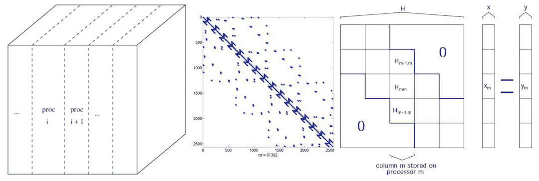
The limiting operation of the Lanczos solver is the complex sparse matrix–vector product. NEMO 3-D cuts the device into slices, one per processor, and communicates only across the slice surfaces. PARPACK was about 10 times slower, and the folded-spectrum method also slower than Lanczos.
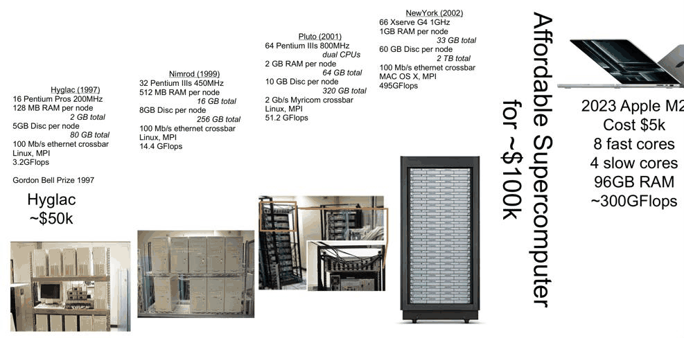
NEMO 3-D grew up on Beowulf clusters built from commodity parts at JPL: from Hyglac (1997, 16 Pentium Pro, 3.2 GFlops, about $50k) to a 495 GFlops Xserve cluster for about $100k (2002). A 2023 laptop delivers about 300 GFlops.
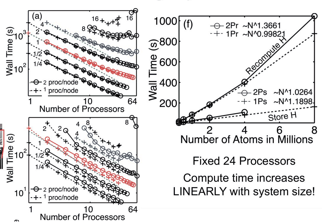
Benchmarks of 2001 (30 Lanczos iterations, ¼ to 16 million atoms): good strong scaling, a second processor per node that slows the code down (memory bandwidth), parallel efficiency of 50–60% when the Hamiltonian is recomputed and 65–80% when it is stored, and a 3–4 times speed-up from storing it.
With the number of processors fixed, the time grows linearly with the number of atoms.
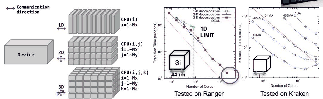
Scaling to 8,192 cores in 2007 used a one-dimensional decomposition, a long thin wire rather than a dot. NEMO 3-D Peta (Sunhee Lee, Hoon Ryu) added 2-D and 3-D decompositions and ran on more than 30,000 cores, from 10 hours to 20 minutes.

In this notebook

Time the open-nemo tight-binding Hamiltonian and its product with a vector against the number of atoms, and estimate the memory of a stored sp3d5s* Hamiltonian.
Put the machines of the lecture next to one another.
Cut a GaAs cube into slabs and into cubes and count, from the actual bonds, how many atoms each domain must receive per product.
Combine the measured product time with the halo sizes in a simple strong-scaling model of the 44 nm silicon cube of slide 13.

Run the notebookEvery number and figure on this page comes from it. Change it, rerun it, take it further.

Download .ipynb View on GitHub

Run it on your own machine

The notebook needs open-nemo (Python ≥ 3.10 and a C++20 compiler; BLAS/LAPACK).

git clone https://github.com/denphi/open-nemo.git && cd open-nemo
python3 -m venv .venv && source .venv/bin/activate
pip install -e ".[notebooks]"
jupyter lab From_Atoms_to_Devices/07_quantum_dots_and_nemo3d/21_5_parallel_computing.ipynb

Code9 lines · cell 1

import time
import numpy as np
import matplotlib.pyplot as plt
import opennemo as nemo
from scipy.spatial import cKDTree
from opennemo.visualization import style
from opennemo.structures.structure import supercell

style.use(notebook=True)

1. The work: one sparse product per Lanczos step#

Slide 2: slicing the domain and the block-tridiagonal matrix — Slide 2: the device is cut into slices, one per processor; ordering the atoms slice by slice makes the Hamiltonian block tridiagonal, and processor $m$ needs from its neighbours only the parts of $\mathbf{x}$ that couple across its two surfaces.

Every Lanczos step (lecture 21.4) is one product $\mathbf{y} = H\mathbf{x}$ plus a few vector operations. With nearest-neighbour tight binding each row of $H$ has a fixed number of non-zeros, so the cost of a product is proportional to the number of atoms. We time it for bulk GaAs supercells in the sp3s* basis (5 orbitals per atom, no spin), together with the time to build $H$.

Code31 lines · cell 3

GAAS = nemo.structures.materials.load("klimeck2002_sp3s")["GaAs"]
lat = nemo.structures.lattice.from_material(GAAS)
rows = []
for n in (4, 6, 8, 10, 12, 14):
    s = supercell(lat, (n, n, n))
    t0 = time.perf_counter()
    H = nemo.models.tb.SlaterKoster(GAAS).build(s).at(np.zeros(3)).tocsr().astype(complex)
    t_build = time.perf_counter() - t0
    x = np.ones(H.shape[0], complex)
    H @ x
    t0 = time.perf_counter()
    for _ in range(20):
        H @ x
    t_mv = (time.perf_counter() - t0) / 20
    rows.append((s.num_atoms, H.shape[0], H.nnz, t_build, t_mv))
    print(f"{s.num_atoms:6d} atoms, {H.shape[0]:6d} rows, {H.nnz:8d} non-zeros: build {t_build:6.3f} s, "
          f"product {t_mv * 1e3:6.3f} ms ({8 * H.nnz / t_mv / 1e9:4.1f} GFlop/s)")
rows = np.array(rows)
atoms, nnz, t_build, t_mv = rows[:, 0], rows[:, 2], rows[:, 3], rows[:, 4]
p_mv = np.polyfit(np.log(atoms), np.log(t_mv), 1)[0]
p_b = np.polyfit(np.log(atoms), np.log(t_build), 1)[0]
ns_per_nnz = np.median(t_mv / nnz) * 1e9
print(f"time ~ N^{p_mv:.2f} (product), N^{p_b:.2f} (build); {ns_per_nnz:.2f} ns per complex non-zero")
print(f"building H costs {np.median(t_build / t_mv):.0f} products")

fig, ax = plt.subplots(figsize=(6, 4))
ax.plot(atoms / 1e3, t_mv * 1e3, "o-", color=style.OPEN_NEMO, label="product H x (ms)")
ax.plot(atoms / 1e3, t_build, "s--", color=style.CONTEXT, label="build H (s)")
ax.set(xlabel="atoms (thousands)", ylabel="time", title="sp3s* GaAs, one core")
ax.legend(frameon=False)
fig.tight_layout()

   512 atoms,   2560 rows,    47616 non-zeros: build  0.020 s, product  0.029 ms (13.3 GFlop/s)
  1728 atoms,   8640 rows,   160704 non-zeros: build  0.067 s, product  0.093 ms (13.9 GFlop/s)
  4096 atoms,  20480 rows,   380928 non-zeros: build  0.165 s, product  0.218 ms (14.0 GFlop/s)
  8000 atoms,  40000 rows,   744000 non-zeros: build  0.327 s, product  0.431 ms (13.8 GFlop/s)
 13824 atoms,  69120 rows,  1285632 non-zeros: build  0.544 s, product  0.760 ms (13.5 GFlop/s)
 21952 atoms, 109760 rows,  2041536 non-zeros: build  0.930 s, product  1.167 ms (14.0 GFlop/s)
time ~ N^0.99 (product), N^1.01 (build); 0.58 ns per complex non-zero
building H costs 738 products

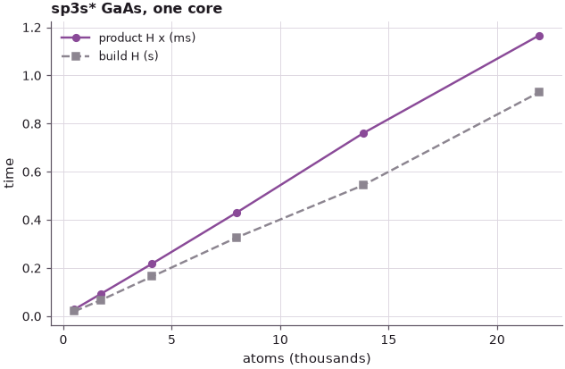
Figure computed by the notebook with open-nemo

Slide 10: compute time against the number of atoms on 24 processors — Slide 10: the 2001 benchmarks. Left, wall time against the number of processors for ¼ to 16 million atoms (top: Hamiltonian recomputed, bottom: stored). Right, with 24 processors fixed, the time grows linearly with the number of atoms.

Both the product and the construction of $H$ grow linearly with the number of atoms, as on slide 10: the fitted exponents are 1.0 within a few hundredths. One complex non-zero costs well under 1 ns on one core of the machine that ran this notebook, 10–14 GFlop/s counting 8 floating-point operations per complex multiply–add (timings vary by a few tens of percent from run to run).

The lecture's "recompute or store" question depends on the code. In NEMO 3-D, recomputing the matrix elements on the fly made the product 3–4 times slower than using a stored matrix (slide 9). open-nemo builds $H$ in vectorized Python, roughly 700 times the cost of a product, so it always stores $H$. What storage costs in memory is the next question:

Code10 lines · cell 5

SPDS = nemo.structures.materials.load("klimeck2002_sp3d5s")["GaAs"]
small = supercell(nemo.structures.lattice.from_material(SPDS), (4, 4, 4))
Hs = nemo.models.tb.SlaterKoster(SPDS, spin=True).build(small).at(np.zeros(3)).tocsr()
nnz_atom = Hs.nnz / small.num_atoms
bytes_atom = nnz_atom * (16 + 4) + 20 * 4                 # complex value + int32 column, row pointers
print(f"sp3d5s* with spin: {Hs.shape[0] // small.num_atoms} rows and {nnz_atom:.0f} non-zeros per atom, "
      f"{bytes_atom / 1e3:.1f} kB per atom stored")
for million in (0.25, 1, 4, 16):
    print(f"{million:5.2f} M atoms: stored H {million * 1e6 * bytes_atom / 1e9:6.1f} GB, "
          f"Lanczos vectors {3 * million * 1e6 * 20 * 16 / 1e9:5.2f} GB")

sp3d5s* with spin: 20 rows and 827 non-zeros per atom, 16.6 kB per atom stored
 0.25 M atoms: stored H    4.2 GB, Lanczos vectors  0.24 GB
 1.00 M atoms: stored H   16.6 GB, Lanczos vectors  0.96 GB
 4.00 M atoms: stored H   66.5 GB, Lanczos vectors  3.84 GB
16.00 M atoms: stored H  266.1 GB, Lanczos vectors 15.36 GB

Sixteen million atoms need 266 GB for the stored sp3d5s* Hamiltonian, against 64 GB of memory in the whole Pluto cluster of 2001 (and 1 GB per processor). That is why NEMO 3-D could also recompute $H$ on the fly, keeping only the Lanczos vectors (15 GB at 16 million atoms), and why the 8 and 16 million-atom systems on slide 5 had to run in parallel just to fit: parallel computing does not only shorten the time, it makes the large systems possible. The memory also explains the second processor per node of slides 4–7: two processors sharing one memory bus that a sparse product already saturates are slower than one.

2. Four generations of Beowulf clusters, and a laptop#

Slide 3: from Hyglac to the 2023 laptop — Slide 3: the JPL clusters on which NEMO 3-D was developed, following the Beowulf concept of Tom Sterling: commodity processors, Ethernet or Myrinet, Linux and MPI.

Code13 lines · cell 7

machines = [  # name, year, processors, peak GFlops, total RAM (GB), cost ($k)
    ("Hyglac", 1997, "16 Pentium Pro 200 MHz", 3.2, 2, 50),
    ("Nimrod", 1999, "32 Pentium III 450 MHz", 14.4, 16, None),
    ("Pluto", 2001, "64 Pentium III 800 MHz", 51.2, 64, None),
    ("NewYork", 2002, "66 Xserve G4 1 GHz", 495, 33, 100),
    ("Apple M2", 2023, "8 + 4 cores", 300, 96, 5),
]
print(f"{'machine':9s} {'year':>4s}  {'processors':24s} {'GFlops':>7s} {'RAM GB':>7s} "
      f"{'GFlops per $1k':>15s}")
for name, year, proc, gf, ram, cost in machines:
    per = f"{gf / cost:15.2f}" if cost else f"{'-':>15s}"
    print(f"{name:9s} {year:4d}  {proc:24s} {gf:7.1f} {ram:7d} {per}")
print(f"\nmeasured above, one core, sparse product: {8 * np.median(nnz / t_mv) / 1e9:.1f} GFlop/s")

machine   year  processors                GFlops  RAM GB  GFlops per $1k
Hyglac    1997  16 Pentium Pro 200 MHz       3.2       2            0.06
Nimrod    1999  32 Pentium III 450 MHz      14.4      16               -
Pluto     2001  64 Pentium III 800 MHz      51.2      64               -
NewYork   2002  66 Xserve G4 1 GHz         495.0      33            4.95
Apple M2  2023  8 + 4 cores                300.0      96           60.00

measured above, one core, sparse product: 13.8 GFlop/s

From Hyglac to the laptop, peak speed per dollar grew by a factor of about 940, from 0.064 to 60 GFlops per $1000. The peak figures overstate what a sparse product achieves, since a product reads 20 bytes for 8 operations and is limited by memory bandwidth, not by arithmetic; the 10–14 GFlop/s measured on one core is a fair figure for the kernel that matters here.

3. Domain decomposition: slabs or cubes#

In the decomposition of slide 2 each processor owns a slab of atoms and its rows of $H$. Before each product it must receive the entries of $\mathbf{x}$ on the halo: the atoms of other domains that are bonded to one of its own. The work of a domain grows with its volume, its communication with its surface. We cut a GaAs cube of $24^3$ conventional cells (13.6 nm, 110,592 atoms) into $P$ slabs along $x$ (1-D) or into $p^3$ cubes (3-D), and count owned and halo atoms from the actual bonds.

Code32 lines · cell 9

cube = supercell(lat, (24, 24, 24))
X = np.asarray(cube.positions)
bonds = cKDTree(X).query_pairs(0.26, output_type="ndarray")      # nearest neighbours, 0.245 nm
bonds = np.vstack([bonds, bonds[:, ::-1]])                       # surface bonds of the open cube cut
lo, hi = X.min(0), X.max(0) + 1e-9
planes = len(np.unique(np.round(X[:, 0], 4)))
print(f"{cube.num_atoms} atoms, {planes} atomic planes along x, "
      f"{len(bonds) / cube.num_atoms:.2f} bonds per atom")


def halo(domain):
    # number of owned and halo atoms of every domain
    i, j = bonds[:, 0], bonds[:, 1]
    cut = domain[i] != domain[j]
    pairs = np.unique(domain[i[cut]].astype(np.int64) * len(X) + j[cut])
    n_dom = domain.max() + 1
    return np.bincount(domain, minlength=n_dom), np.bincount(pairs // len(X), minlength=n_dom)


dec = {"1-D slabs": [], "3-D cubes": []}
for P in (2, 4, 8, 16, 32, 48, 96, 192):
    d = np.floor((X[:, 0] - lo[0]) / (hi[0] - lo[0]) * P).astype(int)
    own, h = halo(d)
    dec["1-D slabs"].append((P, own.min(), own.max(), h.max()))
for p in (2, 3, 4, 6, 8, 12):
    c = np.floor((X - lo) / (hi - lo) * p).astype(int)
    own, h = halo(c[:, 0] * p * p + c[:, 1] * p + c[:, 2])
    dec["3-D cubes"].append((p**3, own.min(), own.max(), h.max()))
for name, r in dec.items():
    print(name)
    for P, omin, omax, hmax in r:
        print(f"  P = {P:5d}: owned {omin:6d}-{omax:6d} atoms, halo {hmax:5d}, halo/owned {hmax / omax:5.2f}")

110592 atoms, 96 atomic planes along x, 3.88 bonds per atom
1-D slabs
  P =     2: owned  55296- 55296 atoms, halo  1152, halo/owned  0.02
  P =     4: owned  27648- 27648 atoms, halo  2303, halo/owned  0.08
  P =     8: owned  13824- 13824 atoms, halo  2303, halo/owned  0.17
  P =    16: owned   6912-  6912 atoms, halo  2304, halo/owned  0.33
  P =    32: owned   3456-  3456 atoms, halo  2304, halo/owned  0.67
  P =    48: owned   2304-  2304 atoms, halo  2304, halo/owned  1.00
  P =    96: owned   1152-  1152 atoms, halo  2304, halo/owned  2.00
  P =   192: owned      0-  1152 atoms, halo  2304, halo/owned  2.00
3-D cubes
  P =     8: owned  13824- 13824 atoms, halo   900, halo/owned  0.07
  P =    27: owned   4096-  4096 atoms, halo   813, halo/owned  0.20
  P =    64: owned   1728-  1728 atoms, halo   465, halo/owned  0.27
  P =   216: owned    512-   512 atoms, halo   213, halo/owned  0.42
  P =   512: owned    216-   216 atoms, halo   123, halo/owned  0.57
  P =  1728: owned     64-    64 atoms, halo    57, halo/owned  0.89

Code10 lines · cell 10

fig, ax = plt.subplots(figsize=(6, 4))
for (name, r), c in zip(dec.items(), (style.CONTEXT, style.OPEN_NEMO)):
    r = np.array([v for v in r if v[1] > 0])
    ax.loglog(r[:, 0], r[:, 3] / r[:, 2], "o-", color=c, label=name)
ax.axvline(planes, color=style.CONTEXT, ls=":", lw=1)
ax.text(planes * 0.9, 0.04, "one plane\nper slab", ha="right", fontsize=8)
ax.set(xlabel="number of domains P", ylabel="halo atoms / owned atoms",
       title=r"GaAs cube $24^3$ cells, 110,592 atoms")
ax.legend(frameon=False)
fig.tight_layout()

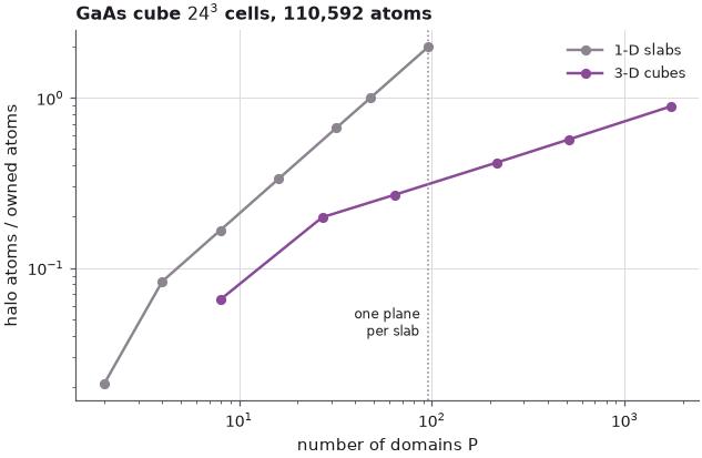
A slab always receives two atomic planes, 2 × 1152 = 2304 atoms here, however thin it is, so the ratio of halo to owned atoms grows linearly with $P$: 0.02 at two slabs, 1.0 at 48 slabs of two planes, 2.0 at 96 slabs of one plane. At 192 slabs some are empty: a 1-D decomposition cannot use more processors than there are atomic planes. Cubes keep a smaller halo: 64 cubes have a ratio of 0.27, against 0.67 for 32 slabs and 1.00 for 48. They can be made almost as small as the unit cell: 1728 cubes of 64 atoms still work, with a halo of 0.89 times the domain.

That is the "cheat" of slide 12: the 8,192-core runs of 2007 used a 1-D decomposition, so the structure had to be a long thin wire with at least 8,192 planes along its axis, not a quantum dot.

4. A strong-scaling model#

Slide 13: 1-D, 2-D and 3-D decompositions in NEMO 3-D Peta — Slide 13: 1-D, 2-D and 3-D decompositions (left); execution time against cores for a 44 nm silicon cube on Ranger, where the 1-D decomposition stops near 100 cores (centre); and Kraken benchmarks from 16 million to one billion atoms (right).

A simple model of one Lanczos step on $P$ processors adds the compute time of a domain to the time to receive its halo:

T(P) = \frac{N}{P}\, t_\text{atom} \;+\; m\,\tau \;+\; \frac{N_\text{halo}\, B \times 16\ \text{bytes}}{b},

with $t_\text{atom}$ the time of one product per atom on one processor, $m$ messages of latency $\tau$ (2 neighbours for slabs, 26 for cubes), $B = 20$ orbitals and bandwidth $b$. The halo sizes come from section 3: a slab receives two atomic planes, a cube one plane on each of its six faces, $6 \times 2\ell^2$ atoms for a side of $\ell$ cells, plus edges (fitted to the counts above). We apply it to the 44 nm silicon cube of slide 13 (sp3d5s* with spin) in two settings:

2001: $t_\text{atom} = 20\ \mu$s, read off slide 10 (24 processors take about 25 s for 30 products of 1 million atoms with a stored $H$), with the 100 Mb/s Ethernet of the cluster and 100 µs latency;
today: $t_\text{atom} = 0.5\ \mu$s, a round value close to the measured time per non-zero times the 827 non-zeros per atom of section 1, with a 100 Gb/s network and 2 µs latency.

The model ignores overlap of computing and communication, memory-bandwidth limits and load imbalance, so it gives the shape of the curves, not measured times.

Code50 lines · cell 13

a_si = 0.5431
L_cells = round(44 / a_si)                                        # 44 nm cube: 81 cells
N = 8 * L_cells**3
planes_si = 4 * L_cells
per_plane = 2 * L_cells**2                                        # atoms in one (100) plane
cub = np.array([(24 / round(P ** (1 / 3)), hmax) for P, _, _, hmax in dec["3-D cubes"][1:]])
c_cube = np.median(cub[:, 1] / cub[:, 0]**2)                      # halo ~ c l^2 (interior cubes)
print(f"44 nm Si cube: {L_cells} cells, {N / 1e6:.2f} M atoms, {planes_si} planes of {per_plane} atoms; "
      f"cube halo ~ {c_cube:.1f} l^2 atoms (l in cells)")

settings = {  # t_atom (s), bandwidth (bytes/s), latency (s)
    "2001": (20e-6, 100e6 / 8, 100e-6),
    "today": (0.5e-6, 100e9 / 8, 2e-6),
}
print(f"t_atom today: 0.5 us assumed; measured in section 1: {nnz_atom * ns_per_nnz * 1e-3:.2f} us")


def step_time(P, kind, t_atom, bw, lat_s):
    if P == 1:
        return N * t_atom
    if kind == "1-D":
        halo_atoms, msgs = 2 * per_plane, 2
    else:
        halo_atoms, msgs = c_cube * (L_cells / P ** (1 / 3))**2, 26
    return N / P * t_atom + msgs * lat_s + halo_atoms * 20 * 16 / bw


P1 = np.unique(np.round(np.logspace(0, np.log10(planes_si), 30)).astype(int))
P3 = np.unique(np.round(np.logspace(0, np.log10(32768), 40)).astype(int))
fig, (a1, a2) = plt.subplots(1, 2, figsize=(11, 4.2))
for (name, prm), ls in zip(settings.items(), ("--", "-")):
    for kind, Ps, c in (("1-D", P1, style.CONTEXT), ("3-D", P3, style.OPEN_NEMO)):
        T = np.array([step_time(P, kind, *prm) for P in Ps])
        a1.loglog(Ps, T, ls, color=c, label=f"{kind}, {name}")
        a2.semilogx(Ps, T[0] / (Ps * T), ls, color=c, label=f"{kind}, {name}")
a1.set(xlabel="processors P", ylabel="time per product (s)", title="44 nm Si cube, sp3d5s* + spin")
a2.set(xlabel="processors P", ylabel="parallel efficiency", ylim=(0, 1.05),
       title="efficiency T(1) / (P T(P))")
a2.axvline(planes_si, color=style.CONTEXT, ls=":", lw=1)
a1.legend(frameon=False, fontsize=8)
fig.tight_layout()

steps = 3000
for name, prm in settings.items():
    T1 = step_time(1, "1-D", *prm)
    print(f"\n{name}: one processor {T1:.2f} s per product, {T1 * steps / 3600:.1f} h for {steps} steps; "
          f"slab halo transfer {2 * per_plane * 20 * 16 / prm[1] * 1e3:.2f} ms")
    for kind, P in (("1-D", 64), ("3-D", 64), ("1-D", planes_si), ("3-D", 1000), ("3-D", 32768)):
        T = step_time(P, kind, *prm)
        print(f"  {kind} P = {P:5d}: efficiency {T1 / (P * T):4.2f}, {steps} steps in {T * steps:8.1f} s")

44 nm Si cube: 81 cells, 4.25 M atoms, 324 planes of 13122 atoms; cube halo ~ 13.3 l^2 atoms (l in cells)
t_atom today: 0.5 us assumed; measured in section 1: 0.48 us

2001: one processor 85.03 s per product, 70.9 h for 3000 steps; slab halo transfer 671.85 ms
  1-D P =    64: efficiency 0.66, 3000 steps in   6001.9 s
  3-D P =    64: efficiency 0.90, 3000 steps in   4412.9 s
  1-D P =   324: efficiency 0.28, 3000 steps in   2803.5 s
  3-D P =  1000: efficiency 0.77, 3000 steps in    330.0 s
  3-D P = 32768: efficiency 0.35, 3000 steps in     22.1 s

today: one processor 2.13 s per product, 1.8 h for 3000 steps; slab halo transfer 0.67 ms
  1-D P =    64: efficiency 0.98, 3000 steps in    101.7 s
  3-D P =    64: efficiency 0.99, 3000 steps in    100.2 s
  1-D P =   324: efficiency 0.91, 3000 steps in     21.7 s
  3-D P =  1000: efficiency 0.97, 3000 steps in      6.6 s
  3-D P = 32768: efficiency 0.54, 3000 steps in      0.4 s

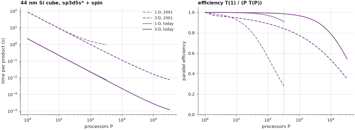
With the 2001 numbers one slab must receive 2 planes of 13,122 atoms, 8.4 MB, which takes 0.67 s on 100 Mb/s Ethernet whatever the number of slabs, while one processor needed 85 s per product. At 64 slabs the efficiency is 0.66, the 50–80% of slides 6 and 8; at the limit of 324 slabs it has fallen to 0.28. In this model cubes would already have done better (0.90 at 64 processors), since their halo shrinks as they get smaller, but slabs are the simplest decomposition to program, need only two messages per product, and suit long structures such as wires.

Today the arithmetic is about 40 times faster per atom and the network 1000 times faster. The 1-D decomposition now runs at 0.91 efficiency at its limit of 324 slabs and cannot go further. The 3-D decomposition goes on: 0.54 efficiency at 32,768 domains of 130 atoms each, and 3000 Lanczos steps in 0.4 s instead of 21.7 s at the 1-D limit, a factor of about 55, the same kind of gain as the "10 hours to 20 minutes" of slide 13.

Summary#

The Lanczos solver spends its time in sparse products $H\mathbf{x}$, linear in the number of atoms; open-nemo's product and Hamiltonian build both scale as $N^{1.0}$.
A stored sp3d5s* Hamiltonian takes about 17 kB per atom: 16 million atoms need 265 GB, more than the whole 2001 cluster, so NEMO 3-D could also recompute $H$ on the fly, and large systems had to run in parallel to fit at all.
A domain receives the atoms bonded to it from its neighbours. A slab's halo is always two atomic planes, so a 1-D decomposition cannot use more processors than planes; cubes have smaller halos and can be divided down to tens of atoms.
A simple model with the product time and the halo sizes reproduces the lecture's picture: with 2001 hardware the slab decomposition gives about 66% efficiency on 64 processors; with today's hardware it is limited by the number of atomic planes, and a 3-D decomposition scales to tens of thousands of cores.

Exercises#

Store the halo counts for 2-D decompositions (cut $x$ and $y$ into $p \times p$ columns) and add them to the plot of section 3. Where do they fall between slabs and cubes?
Repeat the timing of section 1 with klimeck2002_sp3d5s and spin=True. How does the time per non-zero change, and how does the model of section 4 change with it?
In the 2001 setting of the model, what network bandwidth makes the 1-D decomposition of the 44 nm cube reach 80% efficiency at 100 slabs? Compare with the 100 Mb/s Ethernet and the 2 Gb/s Myricom network of slide 3.
Weak scaling: keep 50,000 atoms per processor and let $P$ and $N$ grow together. What does the model predict for the time per step with slabs and with cubes?