

Lecture 22.1
Optical matrix elements — the dipole matrix element
In the lecture
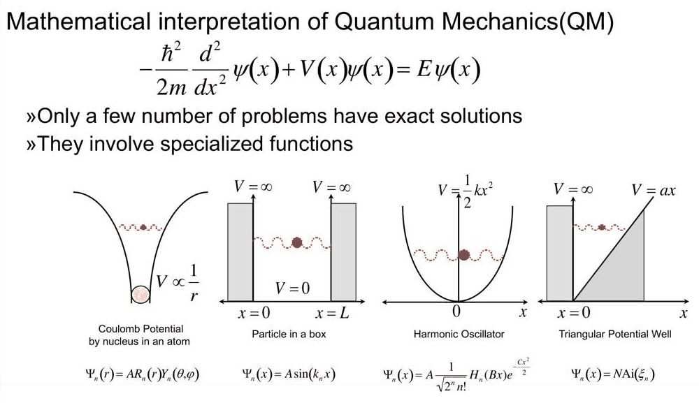
- The few potentials whose Schrödinger equation has closed-form solutions, and the particle in a box as the reference system of the section.
- Light acting on a nanostructure as a spatially uniform electric field that oscillates in time (the dipole, or long-wavelength, approximation), and the interaction Hamiltonian \(H'(t) = e\mathcal{E}(t)\,x\).
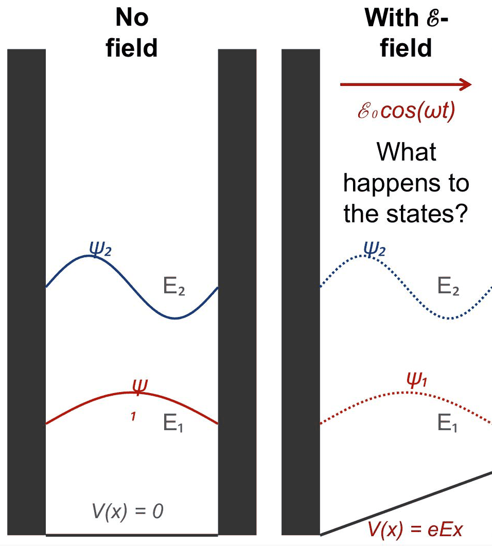
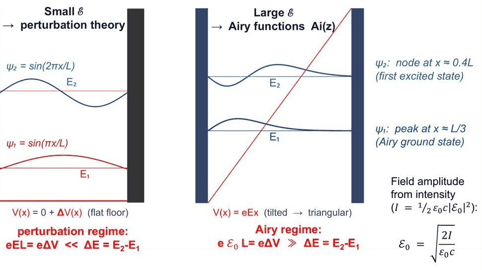
- Two regimes: a weak field that only perturbs the box states, and a strong field that tilts the well into a triangle whose states are Airy functions.
- How strong optical fields really are, from sunlight to femtosecond lasers, against the field at which a 10 nm GaAs well leaves the perturbative regime.
- The key equations: the dipole matrix element, Fermi's golden rule and the Einstein A coefficient.
In this notebook
you solve the 10 nm GaAs box with open-nemo's effective-mass model, tilt it with static fields from sunlight strength to beyond the Airy threshold, measure how much the states deform against perturbation theory and against the Airy solution, convert laser intensities into fields, and evaluate the dipole matrix element, the oscillator strength, the spontaneous emission rate and the golden-rule rate of the 1 → 2 transition, checking the position matrix element against the library's velocity operator.
Run it on your own machine
The notebook needs open-nemo (Python ≥ 3.10 and a C++20 compiler; BLAS/LAPACK).
git clone https://github.com/denphi/open-nemo.git && cd open-nemo
python3 -m venv .venv && source .venv/bin/activate
pip install -e ".[notebooks]"
jupyter lab From_Atoms_to_Devices/08_optical_matrix_elements/22_1_dipole_matrix_element.ipynbCode
import numpy as np
import matplotlib.pyplot as plt
from scipy.linalg import eigh_tridiagonal
from scipy.special import airy, ai_zeros
import opennemo as nemo
from opennemo.core import units
from opennemo.simulations import optics
from opennemo.visualization import style

style.use(notebook=True)
1. Analytically solvable problems and the particle in a box#
The lecture opens with a reminder from earlier sections: the one-dimensional Schrödinger equation
has exact solutions for only a handful of potentials \(V(x)\), and each of them comes with its own special functions. The Coulomb potential of a nucleus, \(V \propto 1/r\), has radial functions times spherical harmonics, \(\psi = R_n(r)\,Y(\theta, \varphi)\); the particle in a box with infinite walls has sines; the harmonic oscillator, \(V = \tfrac12 k x^2\), has Hermite polynomials times a Gaussian; and the triangular well, \(V = a x\) against a hard wall, has Airy functions \(\mathrm{Ai}\). Two of them, the box and the triangle, return in this lecture.
In three dimensions a box with infinite walls separates into three one-dimensional boxes:
with \(n_x, n_y, n_z = 1, 2, 3, \dots\) The question of the section is the one drawn on slide 4: what happens when an electron makes a transition between two of these levels, absorbing or emitting a photon of energy \(h\nu\)?
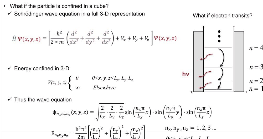
Because the box separates, a field along \(x\) only couples states that differ in \(n_x\); we can work with
the one-dimensional box. Below it is open-nemo's effective-mass model (Heterostructure1D) of a
10 nm GaAs layer (\(m^* = 0.067\,m_0\)) with hard walls. The model puts its sites at \((j + \tfrac12)\Delta\)
and the wave function vanishes one spacing beyond the last site, so a layer \(L - \Delta\) thick is a box
exactly \(L\) wide. We centre it, with the walls at \(x = \pm L/2\), which the next lecture needs.
Code
M, L, DX = 0.067, 10.0, 0.02          # GaAs electron mass (m0), well width and grid spacing (nm)
H2M0 = units.HBAR2_2M0                 # ħ²/2m0 = 0.0381 eV nm²
gaas = nemo.structures.materials.EffectiveMassMaterial("GaAs", M, 12.9)


def box(width=L, field=0.0, num=10, dx=DX):
    """Hard-wall GaAs box `width` nm wide (walls at ±width/2), its floor tilted by a static field
    (V/nm): device, centred grid x (nm), lowest `num` energies (eV) and states ψ (1/√nm, columns)."""
    dev = nemo.Heterostructure1D([nemo.Layer(gaas, width - dx)], spacing=dx)
    x = dev.x + dx / 2 - width / 2     # ψ = 0 one spacing beyond the end sites: walls at ±width/2
    h = dev.hamiltonian.sparse.matrices[0].real
    u = field * (x + width / 2)        # potential energy eℰ(x + L/2) in eV: zero at the left wall
    e, psi = eigh_tridiagonal(h.diagonal() + u, h.diagonal(1), select="i", select_range=(0, num - 1))
    psi = psi / np.sqrt(dx)
    psi *= np.sign(psi[np.argmax(np.abs(psi), axis=0), np.arange(num)])   # largest lobe positive
    return dev, x, e, psi


dev, x, e0, psi0 = box()
e_box = H2M0 * np.pi**2 / (M * L**2) * np.arange(1, 5) ** 2   # ħ²π²n²/(2m*L²)
print(f"{dev.num_sites} sites, walls at x = ±{L / 2} nm")
print(" n   open-nemo (meV)   ħ²π²n²/2m*L² (meV)")
for n in range(4):
    print(f"{n + 1:2d}   {1e3 * e0[n]:12.2f}   {1e3 * e_box[n]:14.2f}")
DE = e0[1] - e0[0]
print(f"E2 - E1 = {1e3 * DE:.1f} meV")
499 sites, walls at x = ±5.0 nm
 n   open-nemo (meV)   ħ²π²n²/2m*L² (meV)
 1          56.12            56.12
 2         224.49           224.50
 3         505.10           505.12
 4         897.94           897.98
E2 - E1 = 168.4 meV
Code
fig, ax = plt.subplots(figsize=(5.5, 4.2))
colours = style.sweep(4)
for n in range(4):
    ax.axhline(1e3 * e0[n], color=colours[n], lw=0.8, ls=":")
    ax.plot(x, 1e3 * e0[n] + 60 * psi0[:, n] / np.abs(psi0[:, n]).max(), color=colours[n])
    ax.text(L / 2 + 0.15, 1e3 * e0[n], f"n = {n + 1}\n{1e3 * e0[n]:.0f} meV", va="center", fontsize=8)
ax.axvspan(-L / 2 - 1.5, -L / 2, color=style.CONTEXT, alpha=0.3, lw=0)
ax.axvspan(L / 2, L / 2 + 2.5, color=style.CONTEXT, alpha=0.3, lw=0)
ax.set(xlim=(-L / 2 - 1.5, L / 2 + 2.5), ylim=(0, 1000), xlabel="position x (nm)",
       ylabel="energy (meV)", title="10 nm GaAs box: levels and ψ (scaled)")
fig.tight_layout()
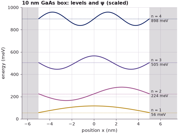
The open-nemo levels agree with \(E_n = \hbar^2\pi^2 n^2/(2m^*L^2)\) to the discretization error of the 0.02 nm grid, and the spacing \(E_2 - E_1 = 3E_1\) is the 168 meV the lecture quotes for this well.
2. Light as a time-dependent electric field: the dipole approximation#
The light is treated "classically", as an electric field. Its wavelength is micrometres (green light, the lecturer's example, is 514 nm), the nanostructure is 5–10 nm. Across the structure the field is therefore spatially uniform: it only goes up and down in time,
which is the dipole, or long-wavelength, approximation. Take the field along \(x\). A uniform field is a linear potential drop, so at every instant the floor of the box is tilted, and the tilt rocks up and down with the field like a lever. For an electron the extra potential energy is the interaction Hamiltonian
with \(e\) the elementary charge (the sign only fixes which way the floor tilts). The lecture's question is what this does to the states: the field shifts the wave functions and couples them, and the coupling drives transitions between states \(i\) and \(f\) when the photon energy matches their difference, \(\hbar\omega \approx |E_f - E_i|\). For small fields the strength of that coupling is measured by the optical (dipole) matrix element
How uniform is "uniform"? The phase of the light wave changes by \(kL = 2\pi n_r L/\lambda\) across a width \(L\), with \(n_r\) the refractive index. For green light in vacuum, and for the infrared photon that the 1 → 2 transition of our well absorbs (inside GaAs, \(n_r \approx 3.3\)):
Code
hc = 1239.84198                        # h c in eV nm
lam_isb = hc / DE                      # wavelength of the 1 -> 2 photon (nm)
print(f"green light, 514 nm, vacuum:        kL = {2 * np.pi * L / 514:.3f} rad")
print(f"1 -> 2 photon, {lam_isb / 1e3:.2f} µm, n_r = 3.3: kL = {2 * np.pi * 3.3 * L / lam_isb:.3f} rad")
green light, 514 nm, vacuum:        kL = 0.122 rad
1 -> 2 photon, 7.36 µm, n_r = 3.3: kL = 0.028 rad
Both phases are small compared with one radian, so the field barely changes across the box: the dipole approximation holds, and best for the infrared transitions between confined levels.
3. Slightly perturbed or fundamentally changed?#
Are the box states only slightly perturbed by the tilt, so that perturbation theory applies, or are they changed into something else? The lecture compares two numbers: the potential drop across the well, \(e\mathcal{E}L\), and the level spacing \(\Delta E = E_2 - E_1\).
- If \(e\mathcal{E}L \ll \Delta E\), the floor is nearly flat, the sines \(\sin(\pi x/L)\) and \(\sin(2\pi x/L)\) are only slightly distorted, and first-order perturbation theory in \(H'\) applies.
- If \(e\mathcal{E}L \gg \Delta E\), the tilt dominates: the well becomes a triangle against one wall, and the states become Airy functions. The slide shows the ground state peaked near \(x \approx L/3\) and the first excited state with its node near \(x \approx 0.4L\), both pushed toward the low wall.
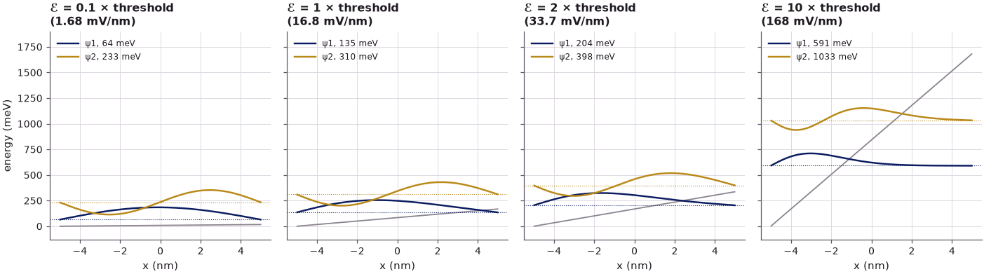
The crossover field is \(\mathcal{E}_\text{thresh} = \Delta E/(eL)\). We tilt the open-nemo box with static fields at fractions and multiples of it. In the triangular limit (right wall far away) the states are
with \(-a_n\) the zeros of \(\mathrm{Ai}\) (\(a_1 = 2.338\), \(a_2 = 4.088\)) and energies measured from the potential at the low wall. The ground state then peaks at \((a_1 - a'_1)\,\ell\) from the wall (\(-a'_1\) the first zero of \(\mathrm{Ai}'\)) and \(\psi_2\) has its node at \((a_2 - a_1)\,\ell\).
Code
F_TH = DE / L                          # threshold field eℰL = ΔE, in V/nm
print(f"threshold field ΔE/(eL) = {F_TH * 1e9:.3g} V/m = {F_TH * 1e9 / 1e6:.1f} MV/m")

mults = (0.1, 1.0, 2.0, 10.0)
fig, axs = plt.subplots(1, 4, figsize=(13, 3.8), sharey=True)
for ax, k in zip(axs, mults):
    F = k * F_TH
    _, _, e, psi = box(field=F)
    ax.plot(x, 1e3 * F * (x + L / 2), color=style.CONTEXT, lw=1.2)
    for n, c in zip((0, 1), style.sweep(2)[::-1]):
        ax.axhline(1e3 * e[n], color=c, lw=0.7, ls=":")
        ax.plot(x, 1e3 * e[n] + 120 * psi[:, n] / np.abs(psi[:, n]).max(), color=c,
                label=f"ψ{n + 1}, {1e3 * e[n]:.0f} meV")
    ax.set(xlabel="x (nm)", title=f"ℰ = {k:g} × threshold\n({F * 1e3:.3g} mV/nm)", ylim=(-130, 1900))
    ax.legend(fontsize=8, loc="upper left", frameon=False)
axs[0].set_ylabel("energy (meV)")
fig.tight_layout()
threshold field ΔE/(eL) = 1.68e+07 V/m = 16.8 MV/m
Code
a = -ai_zeros(2)[0]                    # a1, a2: Ai(-a_n) = 0
a1p = -ai_zeros(1)[1][0]               # a'1: Ai'(-a'1) = 0
print(" ℰ/thresh   ℰ (MV/m)  ψ1 peak (L)  ψ2 node (L) | Airy: peak  node (L)   1 - |<ψ1(0)|ψ1(ℰ)>|²")
for k in (0.1, 0.5, 1.0, 2.0, 3.0, 5.0, 10.0):
    F = k * F_TH
    _, _, e, psi = box(field=F)
    peak = (x[np.argmax(psi[:, 0])] + L / 2) / L
    j = np.nonzero(np.diff(np.sign(psi[:, 1])))[0][0]
    node = (x[j] - psi[j, 1] * DX / (psi[j + 1, 1] - psi[j, 1]) + L / 2) / L
    ell = (H2M0 / (M * F)) ** (1 / 3)
    change = 1 - (np.sum(psi[:, 0] * psi0[:, 0]) * DX) ** 2
    print(f"{k:8.1f}   {F * 1e3:8.1f}   {peak:9.3f}   {node:10.3f}  | {(a[0] - a1p) * ell / L:9.3f}"
          f"  {(a[1] - a[0]) * ell / L:6.3f}   {change:12.3g}")
 ℰ/thresh   ℰ (MV/m)  ψ1 peak (L)  ψ2 node (L) | Airy: peak  node (L)   1 - |<ψ1(0)|ψ1(ℰ)>|²
     0.1        1.7       0.488        0.495  |     0.919   1.219       0.000324
     0.5        8.4       0.446        0.477  |     0.537   0.713        0.00799
     1.0       16.8       0.400        0.454  |     0.426   0.566         0.0306
     2.0       33.7       0.334        0.413  |     0.338   0.449          0.104
     3.0       50.5       0.294        0.379  |     0.296   0.392          0.191
     5.0       84.2       0.250        0.328  |     0.249   0.331          0.344
    10.0      168.4       0.198        0.262  |     0.198   0.263          0.566
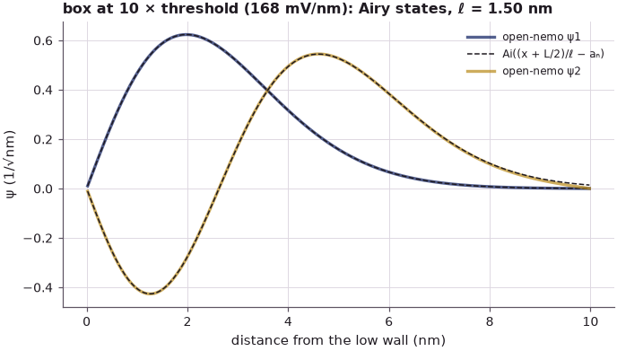
At a tenth of the threshold the states are still the sines: the peak of \(\psi_1\) has moved from the centre only to \(0.49L\), the node of \(\psi_2\) to \(0.495L\), and \(\psi_1\) has changed by three parts in \(10^4\). At twice the threshold the ground state peaks at \(L/3\) and \(\psi_2\) has its node at \(0.41L\): these are the numbers on slide 6, so the slide's Airy picture is a box at about \(2\,\mathcal{E}_\text{thresh}\). From three times the threshold on, the open-nemo ground-state peak agrees with the triangular-well (Airy) value within \(0.002L\), and from five times on the node of \(\psi_2\) does too (the excited state extends further and feels the far wall longer): the states no longer see the second wall. The same comparison for the whole wave functions at ten times the threshold, where the energies agree to 0.2 meV:
Code
F = 10 * F_TH
_, _, e, psi = box(field=F)
ell = (H2M0 / (M * F)) ** (1 / 3)
fig, ax = plt.subplots(figsize=(6.5, 3.8))
for n, c in zip((0, 1), style.sweep(2)[::-1]):
    ai = airy((x + L / 2) / ell - a[n])[0]
    ai /= np.sqrt(np.sum(ai**2) * DX)
    ax.plot(x + L / 2, psi[:, n], color=c, lw=2.2, alpha=0.7, label=f"open-nemo ψ{n + 1}")
    ax.plot(x + L / 2, np.sign(ai[np.argmax(np.abs(ai))]) * ai, "--", color=style.REFERENCE, lw=1,
            label="Ai((x + L/2)/ℓ − aₙ)" if n == 0 else None)
    print(f"ψ{n + 1}: E = {1e3 * e[n]:.1f} meV, Airy aₙ eℰℓ = {1e3 * a[n] * F * ell:.1f} meV")
ax.set(xlabel="distance from the low wall (nm)", ylabel="ψ (1/√nm)",
       title=f"box at 10 × threshold ({F * 1e3:.0f} mV/nm): Airy states, ℓ = {ell:.2f} nm")
ax.legend(fontsize=8, frameon=False)
fig.tight_layout()
ψ1: E = 590.6 meV, Airy aₙ eℰℓ = 590.6 meV
ψ2: E = 1032.9 meV, Airy aₙ eℰℓ = 1032.7 meV
4. How strong are optical fields?#
Which regime does light put us in? The field amplitude follows from the intensity \(I\) of a plane wave, \(I = \tfrac12\varepsilon_0 c\,\mathcal{E}_0^2\), so
The lecture's ladder runs from sunlight (about 1 kW/m², a field of about 900 V/m) through milliwatt and watt continuous-wave (CW) lasers focused to a 10 µm spot, to pulsed femtosecond lasers at 1 GW/cm² (87 MV/m) and the 1 TW/cm² of high-harmonic generation (2.7 GV/m). For the 10 nm GaAs well, \(\Delta E = 168\) meV gives the threshold \(\mathcal{E}_\text{thresh} = \Delta E/(eL) \approx 17\) MV/m. We recompute the ladder, taking a 10 µm spot to be a disc 10 µm in diameter:
Code
def field(intensity):                  # W/m² -> peak field (V/m)
    return np.sqrt(2 * intensity / (units.EPS0 * units.C_LIGHT))


spot = np.pi * (5e-6) ** 2             # 10 µm diameter (m²)
sources = {                            # name: (intensity W/m², field on slide 7 in V/m)
    "sunlight / LED, 1 kW/m²": (1e3, 868),
    "1 mW CW, 10 µm spot": (1e-3 / spot, 98e3),
    "1 W CW, 10 µm spot": (1.0 / spot, 978e3),
    "100 W CW, 10 µm spot": (100.0 / spot, 9.8e6),
    "fs pulse, 1 GW/cm²": (1e13, 86.8e6),
    "HHG, 1 TW/cm²": (1e16, 2.7e9),
}
print(f"{'source':26s} {'I (W/m²)':>10s} {'ℰ0 (V/m)':>10s} {'slide 7':>9s}  ℰ0 / ℰ_thresh")
for name, (i, slide) in sources.items():
    print(f"{name:26s} {i:10.3g} {field(i):10.3g} {slide:9.3g}  {field(i) / (F_TH * 1e9):10.3g}")
p_th = spot * units.EPS0 * units.C_LIGHT * (F_TH * 1e9) ** 2 / 2
print(f"CW power that reaches the threshold in a 10 µm spot: {p_th:.0f} W")
source                       I (W/m²)   ℰ0 (V/m)   slide 7  ℰ0 / ℰ_thresh
sunlight / LED, 1 kW/m²         1e+03        868       868    5.16e-05
1 mW CW, 10 µm spot          1.27e+07   9.79e+04   9.8e+04     0.00582
1 W CW, 10 µm spot           1.27e+10    3.1e+06  9.78e+05       0.184
100 W CW, 10 µm spot         1.27e+12    3.1e+07   9.8e+06        1.84
fs pulse, 1 GW/cm²              1e+13   8.68e+07  8.68e+07        5.16
HHG, 1 TW/cm²                   1e+16   2.74e+09   2.7e+09         163
CW power that reaches the threshold in a 10 µm spot: 30 W
Sunlight, the milliwatt laser and the femtosecond and HHG pulses reproduce the slide. The two watt-class CW lines come out \(\sqrt{10} \approx 3.2\) times higher than on the slide, whose values correspond to a spot about 32 µm across (or ten times less power). With a 10 µm-diameter spot the 100 W line lies at 1.8 times the threshold instead of below it: a CW laser reaches the threshold at about 30 W in such a spot. Sunlight and milliwatt lasers stay four to five orders of magnitude below it, a 1 W laser at 0.18 of it.
How much does each field actually deform the ground state? We tilt the open-nemo box statically with each field and measure \(1 - |\langle\psi_1(0)|\psi_1(\mathcal{E})\rangle|^2\), the weight the state moves out of the unperturbed \(\psi_1\), as the sum of its weights on all other unperturbed states (which keeps the tiny values accurate). First-order perturbation theory gives
Code
dev_all, _, e_all, psi_all = box(num=dev.num_sites)       # every state of the flat box
x1n = psi_all.T @ (x * psi_all[:, 0]) * DX                # <ψn|x|ψ1> (nm)
pt = np.sum((x1n[1:] / (e_all[1:] - e_all[0])) ** 2)     # perturbation theory per (V/nm)²

fields = np.logspace(2.5, 9.7, 49)                        # V/m
change = []
for F in fields * 1e-9:                                   # V/nm
    _, _, e, psi = box(field=F, num=1)
    w = psi_all.T @ psi[:, 0] * DX                         # components on the flat-box states
    change.append(np.sum(w[1:] ** 2))
change = np.array(change)

fig, ax = plt.subplots(figsize=(7.5, 4.4))
ax.loglog(fields, change, color=style.OPEN_NEMO, lw=2, label="open-nemo, tilted box")
ax.loglog(fields, pt * (fields * 1e-9) ** 2, "--", color=style.NEMO_FAMILY, lw=1,
          label="1st-order perturbation theory")
ax.axvline(F_TH * 1e9, color=style.REFERENCE, ls="--", lw=1)
ax.text(F_TH * 1e9 * 1.15, 2e-12, "eℰL = ΔE", color=style.REFERENCE, fontsize=8, rotation=90)
ax.axvspan(F_TH * 1e9, fields[-1], color=style.CONTEXT, alpha=0.12, lw=0)
for name, (i, _) in sources.items():
    f0 = field(i)
    c = np.interp(np.log(f0), np.log(fields), np.log(change))
    ax.plot(f0, np.exp(c), "o", color=style.CONTEXT, ms=5)
    off = (-8, -14) if f0 > F_TH * 1e9 else (-6, 6)        # below the curve beyond the threshold
    ax.annotate(name, (f0, np.exp(c)), xytext=off, textcoords="offset points", fontsize=7, ha="right")
ax.set(xlabel="field amplitude ℰ (V/m)", ylabel="1 − |⟨ψ₁(0)|ψ₁(ℰ)⟩|²", ylim=(1e-13, 3),
       title="deformation of the ground state of a 10 nm GaAs box")
ax.legend(fontsize=8, loc="lower right", frameon=False)
fig.tight_layout()
for name, (i, _) in sources.items():
    f0 = field(i)
    print(f"{name:26s} deformation {np.exp(np.interp(np.log(f0), np.log(fields), np.log(change))):.2g}"
          f"  (perturbation theory {pt * (f0 * 1e-9) ** 2:.2g})")
sunlight / LED, 1 kW/m²    deformation 8.6e-11  (perturbation theory 8.6e-11)
1 mW CW, 10 µm spot        deformation 1.1e-06  (perturbation theory 1.1e-06)
1 W CW, 10 µm spot         deformation 0.0011  (perturbation theory 0.0011)
100 W CW, 10 µm spot       deformation 0.09  (perturbation theory 0.11)
fs pulse, 1 GW/cm²         deformation 0.35  (perturbation theory 0.86)
HHG, 1 TW/cm²              deformation 0.96  (perturbation theory 8.6e+02)
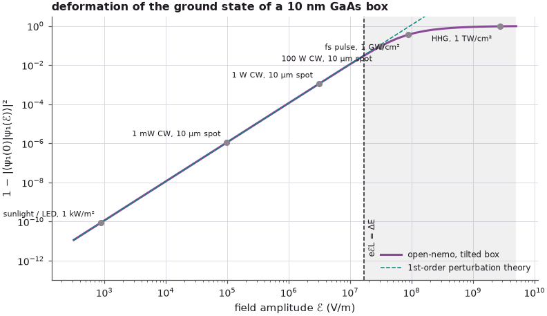
The deformation grows as \(\mathcal{E}^2\) and follows perturbation theory over ten orders of magnitude. For sunlight the ground state changes by about \(10^{-10}\), for a milliwatt laser by \(10^{-6}\) and for a 1 W laser by \(10^{-3}\), exactly as first-order perturbation theory predicts. At the 100 W line (about twice the threshold) the estimate is 20 % high, and it fails for the pulsed lasers (0.86 against 0.35 for the femtosecond pulse; for HHG it exceeds 1 by far), whose fields put the states into the Airy regime of section 3. A static tilt is the lecture's way of judging the regime: in the light wave the tilt rocks at frequency \(\omega\), and section 5 gives the corresponding resonant measure.
This is the lecture's conclusion: for sunlight through focused CW lasers \(\mathcal{E} \ll \mathcal{E}_\text{thresh}\), the unperturbed \(\sin(n\pi x/L)\) states stay valid, and the coupling is described by the dipole matrix element between them. Only intense pulsed lasers reach the Airy regime.
5. Key equations: dipole matrix element, golden rule, spontaneous emission#
The lecture collects the equations that follow from \(H'(t) = e\mathcal{E}_0\cos(\omega t)\,x\) in first-order time-dependent perturbation theory:
- Dipole (optical) matrix element: \(\mu_{if} = e\langle\psi_i|x|\psi_f\rangle = e\int dx\,\psi_i\,x\,\psi_f\).
- Transition rate (Fermi's golden rule with the rotating-wave approximation, which keeps the resonant half \(e\mathcal{E}_0 x/2\) of the cosine): \[W_{if} = \frac{2\pi}{\hbar}\left(\frac{e\mathcal{E}_0}{2}\right)^2|\langle\psi_i|x|\psi_f\rangle|^2\, \delta(E_f - E_i - \hbar\omega) = \frac{\pi}{2\hbar}(e\mathcal{E}_0)^2|\langle\psi_i|x|\psi_f\rangle|^2\, \delta(E_f - E_i - \hbar\omega).\] (Slide 8 writes the prefactor as \(\frac{\pi}{2\hbar}(e\mathcal{E}_0/2)^2\), a factor 4 below the golden rule with \(|V_{fi}| = e\mathcal{E}_0|x_{if}|/2\); we use the form above.)
- Spontaneous emission rate (Einstein A coefficient), in a medium of refractive index \(n_r\): \[A_{if} = \frac{n_r e^2\omega^3}{3\pi\varepsilon_0\hbar c^3}\,|\langle\psi_i|x|\psi_f\rangle|^2 .\]
Every one of them goes through \(|\langle\psi_i|x|\psi_f\rangle|^2\). For the 1 → 2 transition of the box we
compute it from the open-nemo states, compare with the analytic \(16L/(9\pi^2)\) that lecture 22.3
derives, and cross-check with the library's velocity operator: optics.velocity builds
\(\hbar v = i[H, x]\) from the Hamiltonian, and between eigenstates
\(\langle i|\hbar v|f\rangle = i(E_i - E_f)\langle i|x|f\rangle\), so \(|x_{if}| = |\langle i|\hbar v|f\rangle|/|E_f - E_i|\).
optics.oscillator_strengths turns the same elements into the oscillator strength
\(f_{if} = |\langle f|\hbar v|i\rangle|^2/[(\hbar^2/2m_0)(E_f - E_i)]\), which for the infinite well is
\(0.961\,m_0/m^*\).
Code
x12 = np.sum(psi0[:, 0] * x * psi0[:, 1]) * DX            # <ψ1|x|ψ2> (nm)
h = dev.hamiltonian.sparse.matrices[0]
tr = optics.transitions(h, optics.velocity(dev.hamiltonian), (-1.0, -0.5), num_conduction=4,
                        num_valence=0)
hv12 = np.sqrt(tr["matrix"][0][0, 1])                       # |<1|ħv_x|2>| (eV nm)
de = tr["energies"][1] - tr["energies"][0]
f12 = optics.oscillator_strengths(tr["energies"], tr["matrix"][0])[0, 1]
print(f"<ψ1|x|ψ2> = {abs(x12):.4f} nm   (16L/9π² = {16 * L / (9 * np.pi**2):.4f} nm)")
print(f"|<1|ħv|2>| / (E2 - E1) = {hv12:.4f} eV nm / {de:.4f} eV = {hv12 / de:.4f} nm")
print(f"dipole moment e<x> = {abs(x12):.2f} e·nm = {abs(x12) * 1e-9 * units.Q / 3.33564e-30:.0f} debye")
print(f"oscillator strength f12 = {f12:.2f}  ->  f12 m*/m0 = {f12 * M:.3f}")
<ψ1|x|ψ2> = 1.8013 nm   (16L/9π² = 1.8013 nm)
|<1|ħv|2>| / (E2 - E1) = 0.3033 eV nm / 0.1684 eV = 1.8013 nm
dipole moment e<x> = 1.80 e·nm = 87 debye
oscillator strength f12 = 14.34  ->  f12 m*/m0 = 0.961
With the matrix element in hand the rates follow. The Einstein A coefficient below takes \(n_r = 3.3\) for GaAs in the mid-infrared. For a light field the resonant coupling energy is the Rabi energy \(\hbar\Omega_R = e\mathcal{E}_0|x_{12}|\); on resonance with a transition broadened into a Lorentzian of full width \(\Gamma\) (the \(\delta\) function becomes \(2/(\pi\Gamma)\) at its peak), the golden rule gives \(W = (e\mathcal{E}_0 x_{12})^2/(\hbar\Gamma)\), valid while the Rabi energy stays below \(\Gamma\). We take \(\Gamma = 10\) meV.
Code
n_r, gamma = 3.3, 0.010                # refractive index, linewidth (eV)
omega = DE / units.HBAR                # rad/s
xm = abs(x12) * 1e-9                   # m
hbar_j = units.HBAR * units.Q          # J s
A21 = n_r * units.Q**2 * omega**3 * xm**2 / (3 * np.pi * units.EPS0 * hbar_j * units.C_LIGHT**3)
print(f"ħω = {1e3 * DE:.1f} meV, ω = {omega:.3g} rad/s, λ = {lam_isb / 1e3:.2f} µm")
print(f"Einstein A21 = {A21:.3g} 1/s, radiative lifetime {1e9 / A21:.0f} ns\n")
print(f"{'source':26s} {'ħΩ_R (meV)':>11s} {'ħΩ_R/Γ':>8s} {'W on resonance (1/s)':>21s}")
for name, (i, _) in list(sources.items())[:5]:
    rabi = field(i) * xm                                     # eℰ0|x12| in eV
    w = rabi**2 / (units.HBAR * gamma)
    print(f"{name:26s} {1e3 * rabi:11.3g} {rabi / gamma:8.2g} {w:21.3g}")
ħω = 168.4 meV, ω = 2.56e+14 rad/s, λ = 7.36 µm
Einstein A21 = 1.94e+07 1/s, radiative lifetime 52 ns

source                      ħΩ_R (meV)   ħΩ_R/Γ  W on resonance (1/s)
sunlight / LED, 1 kW/m²        0.00156  0.00016              3.71e+05
1 mW CW, 10 µm spot              0.176    0.018              4.73e+09
1 W CW, 10 µm spot                5.58     0.56              4.73e+12
100 W CW, 10 µm spot              55.8      5.6              4.73e+14
fs pulse, 1 GW/cm²                 156       16              3.71e+15
The open-nemo matrix element is \(|x_{12}| = 1.80\) nm, \(0.18L\), equal to \(16L/(9\pi^2)\) to the grid error, and the velocity route of the library gives the same number. The oscillator strength \(f_{12}m^*/m_0 = 0.96\) is the infinite-well value. Spontaneous emission on this 168 meV transition is slow, about 50 ns (in a real GaAs well the upper level empties far faster by emitting optical phonons, which this lecture does not treat). Under illumination, the Rabi energy of a milliwatt laser is a fraction of a meV, below the 10 meV linewidth, and the golden rule applies; at the watt level the Rabi energy approaches the linewidth and the golden-rule rate overestimates, an issue of the resonant drive that appears long before the static Airy threshold.
Summary#
- Only a few potentials have exact solutions; the particle in a box (\(\sin\)) and the triangular well (Airy functions) bracket the problem of a box in a field. For the 10 nm GaAs box (\(m^* = 0.067\,m_0\)) open-nemo gives \(E_2 - E_1 = 168\) meV.
- Light of micrometre wavelength is nearly uniform across a nanostructure (phase change across 10 nm: 0.12 rad for green light, 0.03 rad for the 7.4 µm photon of the 1 → 2 transition): it acts as \(H'(t) = e\mathcal{E}_0\cos(\omega t)\,x\), a floor tilt that rocks in time.
- The perturbative regime holds while \(e\mathcal{E}L \ll \Delta E\); for the 10 nm GaAs well the threshold is \(\Delta E/(eL) = 17\) MV/m. At twice that the states look like slide 6 (\(\psi_1\) peak at \(L/3\), \(\psi_2\) node at \(0.41L\)), and from about three times on they are Airy functions.
- Optical fields from sunlight (870 V/m) to a 1 W CW laser in a 10 µm spot (3.1 MV/m) stay below the threshold; the ground state deforms by \(\sim 10^{-10}\) (sunlight) to \(\sim 10^{-3}\) (1 W), as perturbation theory predicts, so the unperturbed sines and the dipole matrix element \(\langle\psi_i|x|\psi_f\rangle\) are the right description.
- The golden-rule rate, the Einstein A coefficient and the oscillator strength all go through \(|\langle\psi_i|x|\psi_f\rangle|^2\); for the 1 → 2 transition it is \(1.80\) nm, the radiative lifetime about 50 ns, and \(f_{12} = 0.96\,m_0/m^*\).
Exercises#
- Repeat the threshold estimate for a 5 nm and a 20 nm GaAs well with
box(width=...). Show that \(\mathcal{E}_\text{thresh} = \Delta E/(eL)\) scales as \(L^{-3}\), and find the CW power that reaches it in a 10 µm spot for each width. - Replace GaAs by InAs (\(m^* = 0.023\,m_0\); edit the material in
box). Does a lighter mass move the threshold up or down, and by how much for \(L = 10\) nm? - Plot the Stark shift of the ground state, \(E_1(\mathcal{E}) - E_1(0) - e\mathcal{E}L/2\), against the
second-order perturbation result \(-\sum_{n\ne1}(e\mathcal{E}x_{1n})^2/(E_n - E_1)\) from
x1n. Where does the second-order formula fail? - The spontaneous emission rate goes as \(\omega^3|x_{12}|^2\). Using
box(width=...), compute \(A_{21}\) for \(L\) = 5, 10 and 20 nm and find the power law in \(L\).
Further reading#
- Lecture 22.2: allowed and forbidden transitions and Lecture 22.3: an analytical expression for the dipole matrix element, the rest of this section.
- Optical transitions and absorption of quantum wells: interband and intersubband absorption with the 8-band k·p model, including the quantum-confined Stark effect in a field.
- How bands emerge: from one quantum well to fifteen:
the effective-mass
Heterostructure1Dused here, with closed and open boxes. - A GaN/AlN quantum dot: strain, polarization field and the quantum-confined Stark effect: a built-in field strong enough to tilt the confinement, as in section 3.
- D. J. Griffiths, Introduction to Quantum Mechanics (Cambridge University Press), chapters on the infinite square well and time-dependent perturbation theory (Fermi's golden rule, spontaneous emission).
- G. Bastard, Wave Mechanics Applied to Semiconductor Heterostructures (Les Éditions de Physique, 1988): quantum wells in electric fields and their optical matrix elements.